Statistical research is very laborious and expensive, so the idea arose of replacing continuous observation with a selective one.

The main purpose of discontinuous observation is to obtain characteristics of the studied statistical population for the surveyed part of it.

Selective observation- This is a method of statistical research, in which the generalized indicators of the population are established only for a separate part on the basis of the provisions of random selection.

With the sampling method, only a certain part of the studied population is studied, while the statistical population to be studied is called the general population.

A sample population or simply a sample can be called a portion of units selected from the general population that will be subjected to statistical research.

The value of the sampling method: with a minimum number of units under study, a statistical study will be carried out in shorter periods of time and with the least cost of funds and labor.

In the general population, the proportion of units that have the trait under study is called the general proportion (denoted by R), and the average value of the studied variable characteristic is the general average (denoted by NS).

In the sample population, the share of the trait under study is called the sample share, or part (denoted by w), the average value in the sample is sample mean.

If during the period of the survey all the rules of its scientific organization are observed, then the sampling method will give rather accurate results, and therefore it is advisable to use this method to check the data of continuous observation.

This method has become widespread in state and non-departmental statistics, because in the study of the minimum number of units under study, it allows you to carefully and accurately conduct a study.

The studied statistical population consists of units with varying characteristics. The composition of the sample population may differ from the composition of the general population; this discrepancy between the characteristics of the sample and the general population is the sampling error.

The errors inherent in sample observation characterize the size of the discrepancy between the data of the sample observation and the entire population. Errors arising in the course of sampling are called errors of representativeness and are divided into random and systematic.

If the sample population does not accurately reproduce the entire population due to the discontinuous nature of the observation, then this is called random errors, and their sizes are determined with sufficient accuracy on the basis of the law of large numbers and the theory of probability.

Systematic errors arise as a result of violation of the principle of randomness in the selection of population units for observation.

2. Types and schemes of selection

The size of the sampling error and methods for its determination depend on the type and scheme of selection.

There are four types of selection for a set of observation units:

1) random;

2) mechanical;

3) typical;

4) serial (nested).

Random sampling- the most common method of selection in a random sample, it is also called the method of drawing lots, in which a ticket with a serial number is prepared for each unit of the statistical population.

Further, the required number of units of the statistical population is randomly selected. Under these conditions, each of them has the same probability of being included in the sample, for example, the draws of winnings, when a certain part of the numbers on which the winnings fall is randomly selected from the total number of issued tickets. At the same time, all numbers are provided with an equal opportunity to get into the sample.

Mechanical selection- this is a method when the entire population is divided into groups of homogeneous volume according to a random criterion, then only one unit is taken from each group.All units of the studied statistical population are preliminarily arranged in a certain order, but depending on the sample size, the required number of units is mechanically selected at a certain interval ...

Typical selection - This is a method in which the statistical population under study is divided according to a significant, typical feature into qualitatively homogeneous, similar groups, then a certain number of units is randomly selected from each of this group, proportional to the specific weight of the group in the entire population.

Typical selection gives more accurate results, since it includes representatives of all typical groups in the sample.

Serial (nested) selection. Whole groups (series, nests), randomly or mechanically selected, are subject to selection. For each such group and series, continuous observation is carried out, and the results are transferred to the entire population.

The sampling accuracy also depends on the selection scheme. The sampling can be carried out according to the scheme of repeated and non-repeating sampling.

Repeated selection. Each selected unit or series is returned to the entire population and can be returned to the sample. This is the so-called returned ball scheme.

Repeated selection. Each surveyed unit is withdrawn and not returned to the aggregate, so it does not get re-examined. This scheme is called the unreturned ball.

Repeat sampling gives more accurate results because for the same sample size, observation covers more units of the studied population.

Combined selection can go through one or more steps. A sample is called one-stage if the units of the population that are selected once are examined.

The sample is called multistage if the selection of the population goes through stages, successive stages, and each stage, stage of selection has its own unit of selection.

Multiphase sampling - at all stages of the sampling, the same sampling unit is maintained, but several stages, phases of sample surveys are carried out, which differ in the breadth of the survey program and the sample size.

The characteristics of the parameters of the general population and the sample population are indicated by the following symbols:

N- the volume of the general population;

n- sample size;

X- general average;

NS- sample mean;

R- general share;

w - selective share;

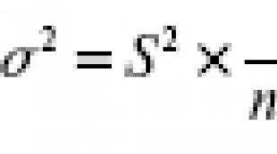
2 - general variance (variance of a feature in the general population);

2 - sample variance of the same feature;

? - standard deviation in the general population;

? - standard deviation in the sample.

3. Sampling errors

Each unit in a sample observation should have an equal opportunity with others to be selected - this is the basis of a self-random sample.

Self-random sampling - This is the selection of units from the entire general population by drawing lots or in another similar way.

The principle of randomness is that the inclusion or exclusion of an object from the sample cannot be influenced by any factor other than case.

Sample share Is the ratio of the number of units in the sample to the number of units in the general population:

Proper random selection in its pure form is the initial one among all other types of selection; it contains and implements the basic principles of selective statistical observation.

The two main types of generalizing indicators that are used in the sampling method are the average value of a quantitative characteristic and the relative value of an alternative characteristic.

The sample fraction (w), or particular, is determined by the ratio of the number of units with the studied feature m, to the total number of units of the sample (n):

To characterize the reliability of sampling indicators, the mean and marginal sampling errors are distinguished.

The sampling error, also called the representativeness error, is the difference between the corresponding sampling and general characteristics:

?x = | x - x |;

?w = | x - p |.

Sampling error is inherent only in sample observations

Sample mean and sample share- these are random variables that take different values ​​depending on the units of the studied statistical population that were included in the sample. Accordingly, sampling errors are also random values ​​and can also take on different values. Therefore, the average of the possible errors is determined - the average sampling error.

The average sampling error is determined by the sample size: the larger the number, other things being equal, the smaller the average sampling error. Covering an increasing number of units of the general population with a sample survey, we more and more accurately characterize the entire general population.

The average sampling error depends on the degree of variation of the studied trait, in turn, the degree of variation is characterized by the variance? 2 or w (l - w)- for an alternative feature. The less the variation of the feature and the variance, the less is the average sampling error, and vice versa.

For random re-sampling, mean errors are theoretically calculated using the following formulas:

1) for the average quantitative trait:

where? 2 - the average value of the variance of the quantitative trait.

2) for a share (alternative feature):

So how is the variance of a trait in the general population? 2 is not known exactly, in practice they use the value of the variance S 2, calculated for the sample population on the basis of the law of large numbers, according to which the sample population with a sufficiently large sample size accurately reproduces the characteristics of the general population.

The formulas for the mean sampling error for random resampling are as follows. For the average value of a quantitative trait: the general variance is expressed through the elective as follows:

where S 2 is the variance value.

Mechanical sampling- this is the selection of units into a sample from the general population, which is divided into equal groups according to a neutral criterion; is done in such a way that only one unit is selected from each such group.

In mechanical selection, the units of the studied statistical population are preliminarily arranged in a certain order, after which a specified number of units are selected mechanically at a certain interval. Moreover, the size of the interval in the general population is equal to the reciprocal of the proportion of the sample.

With a sufficiently large population, mechanical selection in terms of the accuracy of the results is close to self-random.Therefore, to determine the average error of mechanical selection, the formulas for self-random non-repetitive sampling are used.

To select units from a heterogeneous population, the so-called typical sampling is used, it is used when all units of the general population can be divided into several qualitatively homogeneous, similar groups according to the characteristics on which the studied indicators depend.

Then, from each typical group, individual selection of units into the sample population is made by a self-random or mechanical sampling.

Typical sampling is usually used when studying complex statistical populations.

Typical sampling gives more accurate results. Typification of the general population ensures the representativeness of such a sample, the representation of each typological group in it, which makes it possible to exclude the influence of intergroup variance on the mean sampling error. Therefore, when determining the average error of a typical sample, the average of intragroup variances is used as an indicator of variation.

Serial sampling involves random selection from a general population of equal-sized groups in order to subject all units to observation in such groups.

Since all units without exception are examined within groups (series), the average sampling error (when selecting series of equal size) depends only on the intergroup (inter-series) variance.

4. Ways of distributing sample results to the general population

Characterization of the general population based on sample results is the ultimate goal of sample observation.

The sampling method is used to obtain characteristics of the general population for certain indicators of the sample. Depending on the objectives of the study, this is carried out by direct recalculation of the sample indices for the general population or by the method of calculating correction factors.

The method of direct recalculation is that with it the indicators of the sample share w or average NS apply to the general population, taking into account the sampling error.

The method of correction factors is used when the purpose of the sampling method is to clarify the results of complete accounting. This method is used to refine the data of the annual census of livestock among the population.

Statistical population- a set of units with mass, typicality, qualitative homogeneity and the presence of variation.

The statistical population consists of materially existing objects (Workers, enterprises, countries, regions), is an object.

Aggregate unit- each specific unit of the statistical population.

One and the same statistical population can be homogeneous in one attribute and heterogeneous in another.

Qualitative uniformity- the similarity of all units of the aggregate for some reason and the dissimilarity for all the rest.

In a statistical population, the differences between one unit of the population and another are often quantitative in nature. Quantitative changes in the values ​​of a characteristic of different units of the population are called variation.

Variation of a feature- a quantitative change in a trait (for a quantitative trait) during the transition from one unit of the population to another.

Sign Is a property, characteristic feature or other feature of units, objects and phenomena that can be observed or measured. Signs are divided into quantitative and qualitative. The variety and variability of the value of the trait in individual units of the population is called variation.

Attributive (qualitative) characteristics do not lend themselves to numerical expression (composition of the population by sex). Quantitative characteristics are numerically expressed (composition of the population by age).

Index- it is a quantitatively summarizing qualitative characteristic of any property of units or a set as a whole in specific conditions of time and place.

Scorecard Is a set of indicators that comprehensively reflect the phenomenon under study.

For example, the salary is studied:

• Feature - wages
• Statistical population - all employees
• Aggregate unit - each employee
• Qualitative homogeneity - accrued wages
• Variation of a sign - a series of numbers

General population and sample from it

The basis is a set of data obtained as a result of measuring one or more features. The actually observed set of objects, statistically represented by a number of observations of a random variable, is sampling, and hypothetically existing (conjectured) - the general population... The general population can be finite (the number of observations N = const) or infinite ( N = ∞), and a sample from the general population is always the result of a limited number of observations. The number of observations forming a sample is called sample size... If the sample size is large enough ( n → ∞) the sample is considered big otherwise it is called a sample limited volume... The sample is considered small if, when measuring a one-dimensional random variable, the sample size does not exceed 30 ( n<= 30 ), and when measuring several ( k) features in multidimensional space, the ratio n To k less than 10 (n / k< 10) ... The sample forms variation range if its members are ordinal statistics, i.e., sample values ​​of a random variable NS are sorted in ascending order (ranked), the values ​​of the feature are called options.

Example... Almost the same randomly selected set of objects - commercial banks of one administrative district of Moscow, can be considered as a sample from the general population of all commercial banks in this district, and as a sample from the general population of all commercial banks in Moscow, as well as a sample from commercial banks of the country and etc.

Basic sampling methods

The reliability of statistical conclusions and meaningful interpretation of the results depends on representativeness sampling, i.e. completeness and adequacy of representation of the properties of the general population, in relation to which this sample can be considered representative. The study of the statistical properties of a population can be organized in two ways: using continuous and discontinuous. Continuous observation foresees a survey of all units studied the aggregate, a discontinuous (selective) observation- only parts of it.

There are five main ways of organizing sample observation:

1. simple random selection, in which objects are randomly extracted from a general population of objects (for example, using a table or a random number generator), with each of the possible samples having equal probability. Such samples are called proper random;

2. easy selection using a regular procedure is carried out using a mechanical component (for example, date, day of the week, apartment number, alphabet letter, etc.) and the samples obtained in this way are called mechanical;

3. stratified selection consists in the fact that the general population of the volume is subdivided into subsets or layers (strata) of the volume so that. Strata are homogeneous objects in terms of statistical characteristics (for example, the population is divided into strata by age groups or social class; enterprises - by industry). In this case, the samples are called stratified(otherwise, stratified, typical, zoned);

4.methods serial selection are used to form serial or nested samples... They are convenient if it is necessary to examine at once a "block" or a series of objects (for example, a consignment of goods, products of a certain series, or the population in the territorial-administrative division of the country). The selection of batches can be carried out in a purely random or mechanical way. At the same time, a complete survey of a certain batch of goods, or an entire territorial unit (residential building or quarter) is carried out;

5. combined(stepwise) selection can combine several methods of selection at once (for example, stratified and random or random and mechanical); such a sample is called combined.

Selection types

By mind distinguish between individual, group and combined selection. At individual selection individual units of the general population are selected into the sample, with group selection- qualitatively homogeneous groups (series) of units, and combined selection assumes a combination of the first and second types.

By method selection distinguish repeated and non-repeated sample.

Nonrepeatable selection is called, in which the unit that got into the sample does not return to the original population and does not participate in the further selection; while the number of units in the general population N is reduced in the selection process. At repeated selection caught in the sample, the unit after registration is returned to the general population and thus retains an equal opportunity, along with other units, to be used in the further selection procedure; while the number of units in the general population N remains unchanged (the method is rarely used in socio-economic research). However, with a large N (N → ∞) formulas for nonrepeatable selections approach those for repeated selection and almost more often the latter are used ( N = const).

The main characteristics of the parameters of the general and sample population

The statistical conclusions of the study are based on the distribution of a random variable, while the observed values (x 1, x 2, ..., x n) are called realizations of the random variable NS(n is the sample size). The distribution of a random variable in the general population is theoretical, ideal, and its sample analogue is empirical distribution. Some theoretical distributions are given analytically, i.e. their options determine the value of the distribution function at each point in the space of possible values ​​of the random variable. For a sample, the distribution function is difficult to determine, and sometimes impossible, therefore options are estimated from empirical data, and then they are substituted into an analytical expression describing the theoretical distribution. In this case, the assumption (or hypothesis) about the type of distribution can be both statistically correct and erroneous. But in any case, the empirical distribution reconstructed from the sample only roughly characterizes the true one. The most important distribution parameters are expected value and variance.

By their nature, distributions are continuous and discrete... The best known continuous distribution is normal... Selective analogs of parameters and for it are: mean value and empirical variance. Among the discrete ones in socio-economic research, the most commonly used alternative (dichotomous) distribution. The parameter of the mathematical expectation of this distribution expresses the relative value (or share) units of the population that have the trait under study (it is indicated by a letter); the proportion of the population that does not have this feature is denoted by the letter q (q = 1 - p)... The variance of the alternative distribution also has an empirical analogue.

The characteristics of the distribution parameters are calculated in different ways depending on the type of distribution and on the method of selecting the units of the population. The main ones for theoretical and empirical distributions are given in table. 1.

Fraction of sample k n is the ratio of the number of units in the sample to the number of units in the general population:

k n = n / N.

Sample fraction w Is the ratio of units with the studied feature x to the sample size n:

w = n n / n.

Example. In a batch of goods containing 1000 units, with a 5% sample sample fraction k n in absolute value is 50 units. (n = N * 0.05); if in this sample 2 defective products are found, then selective waste rate w will be 0.04 (w = 2/50 = 0.04 or 4%).

Since the sample population is different from the general population, then sampling errors.

Table 1. Basic parameters of the general and sample population

Sampling errors

For any (solid and selective) errors of two types may occur: registration and representativeness. Errors registration can have random and systematic character. Random errors are made up of many different uncontrollable causes, are unintentional and usually balance each other in aggregate (for example, changes in instrument readings due to temperature fluctuations in the room).

Systematic errors are tendentious, since they violate the rules for selecting objects in the sample (for example, deviations in measurements when changing the setting of the measuring device).

Example. To assess the social status of the population in the city, it is planned to examine 25% of families. If, at the same time, the choice of every fourth apartment is based on its number, then there is a danger of selecting all apartments of only one type (for example, one-room apartments), which will provide a systematic error and distort the results; the choice of the apartment number by lot is more preferable, since the error will be accidental.

Representative errors are inherent only to selective observation, they cannot be avoided and they arise as a result of the fact that the sample does not fully reproduce the general population. The values ​​of the indicators obtained from the sample differ from the indicators of the same values ​​in the general population (or obtained through continuous observation).

Sample observation error is the difference between the value of the parameter in the general population and its sample value. For the average value of a quantitative characteristic, it is equal to:, and for a share (alternative characteristic) -.

Sampling errors are characteristic only of sample observations. The larger these errors are, the more the empirical distribution differs from the theoretical one. The parameters of the empirical distribution are random values, therefore, sampling errors are also random values, they can take different values ​​for different samples, and therefore it is customary to calculate average error.

Average sampling error there is a value that expresses the standard deviation of the sample mean from the mathematical expectation. This value, subject to the principle of random selection, depends primarily on the sample size and on the degree of variation of the feature: the greater and the less the variation of the feature (and hence the value), the smaller the value of the average sampling error. The ratio between the variances of the general and sample populations is expressed by the formula:

those. for sufficiently large, we can assume that. The average sampling error shows the possible deviations of the parameter of the sample population from the parameter of the general population. Table 2 shows expressions for calculating the average sampling error for different methods of organizing observation.

Table 2. Mean error (m) of sample mean and proportion for different types of sample

Where is the average of the intragroup sample variances for a continuous feature;

Average of intra-group share variances;

- number of selected series, - total number of series;

,

where is the average of the -th series;

- the overall average for the entire sample for a continuous feature;

,

where is the share of the feature in the th series;

- the total share of the feature in the entire sample.

However, the value of the average error can be judged only with a certain, probability P (P ≤ 1). Lyapunov A.M. proved that the distribution of sample means, and hence their deviations from the general average, for a sufficiently large number approximately obeys the normal distribution law, provided that the general population has a finite average and limited variance.

Mathematically, this statement for the mean is expressed as:

and for the fraction, expression (1) will take the form:

where - there is marginal sampling error, which is a multiple of the mean sampling error , and the factor of multiplicity is the Student's test ("confidence factor") proposed by the US. Gosset (alias "Student"); values ​​for different sample sizes are stored in a special table.

The values ​​of the function Ф (t) for some values ​​of t are equal:

Therefore, expression (3) can be read as follows: with probability P = 0.683 (68.3%) it can be argued that the difference between the sample and general mean will not exceed one value of the mean error m (t = 1), with probability P = 0.954 (95.4%)- that it will not exceed the value of two mean errors m (t = 2), with probability P = 0.997 (99.7%)- will not exceed three values m (t = 3). Thus, the probability that this difference will exceed three times the value of the mean error determines error level and is no more 0,3% .

Table 3 shows the formulas for calculating the marginal sampling error.

Table 3. Marginal error (D) of the sample for the mean and proportion (p) for different types of sample observation

Distribution of sample results to the general population

The ultimate goal of selective observation is to characterize the general population. For small sample sizes, empirical estimates of the parameters (and) can significantly deviate from their true values ​​(and). Therefore, it becomes necessary to establish the boundaries within which the true values ​​(and) lie for the sample values ​​of the parameters (and).

Confidence interval of any parameter θ of the general population is called a random range of values ​​of this parameter, which with a probability close to 1 ( reliability) contains the true value of this parameter.

Marginal error sampling Δ allows you to determine the limit values ​​of the characteristics of the general population and their confidence intervals which are equal:

Bottom line confidence interval obtained by subtracting marginal error from the sample mean (share), and the upper one by adding it.

Confidence interval for the mean, it uses the marginal sampling error and for a given confidence level is determined by the formula:

This means that with a given probability R, which is called the confidence level and is uniquely determined by the value t, it can be argued that the true value of the mean lies in the range from , and the true value of the fraction is in the range from

When calculating the confidence interval for three standard confidence levels P = 95%, P = 99% and P = 99.9% the value is selected by. Applications depending on the number of degrees of freedom. If the sample size is large enough, then the values ​​corresponding to these probabilities t are equal: 1,96, 2,58 and 3,29 ... Thus, the marginal sampling error makes it possible to determine the limiting values ​​of the characteristics of the general population and their confidence intervals:

The distribution of the results of selective observation to the general population in socio-economic research has its own characteristics, since it requires the completeness of the representativeness of all its types and groups. The basis for the possibility of such distribution is the calculation relative error:

where Δ % - relative marginal sampling error; ,.

There are two main methods of extending sample observation to the general population: direct conversion and method of coefficients.

The essence direct conversion consists in multiplying the sample mean value !! \ overline (x) by the size of the general population.

Example... Let the average number of toddlers in the city be estimated by a sample method and be a person. If there are 1000 young families in the city, then the number of required places in municipal nurseries is obtained by multiplying this average by the size of the general population N = 1000, i.e. will amount to 1200 places.

Odds method it is advisable to use in the case when selective observation is carried out in order to clarify the data of continuous observation.

In this case, the formula is used:

where all the variables are the population size:

Required sample size

Table 4. Required sample size (n) for different types of organization of sample observation

When planning a sample observation with a predetermined value of the admissible sampling error, it is necessary to correctly estimate the required sample size... This volume can be determined on the basis of the permissible error in sample observation based on a given probability that guarantees the permissible value of the error level (taking into account the way of organizing the observation). Formulas for determining the required sample size n are easy to obtain directly from the formulas for the marginal sampling error. So, from the expression for the marginal error:

the sample size is directly determined n:

This formula shows that with decreasing marginal sampling error Δ the required sample size increases significantly, which is proportional to the variance and the square of the Student's test.

For a specific method of organizing observation, the required sample size is calculated according to the formulas given in table. 9.4.

Practical calculation examples

Example 1. Calculation of the mean and the confidence interval for a continuous quantitative characteristic.

To assess the speed of settlement with creditors, the bank carried out a random sample of 10 payment documents. Their values ​​turned out to be equal (in days): 10; 3; 15; 15; 22; 7; eight; 1; 19; twenty.

Necessary with probability P = 0.954 determine the marginal error Δ sample mean and confidence limits for mean time of calculations.

Solution. The average value is calculated using the formula from the table. 9.1 for a sample

The variance is calculated by the formula from table. 9.1.

The mean square error of the day.

The mean error is calculated by the formula:

those. the average is x ± m = 12.0 ± 2.3 days.

The reliability of the mean was

The limiting error is calculated by the formula from table. 9.3 for re-sampling, since the size of the population is unknown, and for P = 0.954 confidence level.

Thus, the average value is equal to `x ± D =` x ± 2m = 12.0 ± 4.6, i.e. its true value ranges from 7.4 to 16.6 days.

Using the Student's table. The application allows us to conclude that for n = 10 - 1 = 9 degrees of freedom, the obtained value is reliable with a significance level of a £ 0.001, i.e. the obtained mean value is significantly different from 0.

Example 2. Estimation of the probability (general share) p.

With a mechanical sampling method of surveying the social status of 1000 families, it was revealed that the share of low-income families was w = 0.3 (30%)(the sample was 2% , i.e. n / N = 0.02). Needed with a level of confidence p = 0.997 determine the indicator R low-income families throughout the region.

Solution. According to the presented values ​​of the function Ф (t) find for a given confidence level P = 0.997 meaning t = 3(see formula 3). Marginal share error w determined by the formula from table. 9.3 for non-repetitive sampling (mechanical sampling is always non-repetitive):

The marginal relative sampling error in % will be:

The probability (general share) of low-income families in the region will be p = w ± Δ w, and the confidence limits p are calculated based on the double inequality:

w - Δ w ≤ p ≤ w - Δ w, i.e. the true value of p lies within:

0,3 — 0,014 < p <0,3 + 0,014, а именно от 28,6% до 31,4%.

Thus, with a probability of 0.997, it can be argued that the share of low-income families among all families in the region ranges from 28.6% to 31.4%.

Example 3. Calculation of the mean and the confidence interval for a discrete feature specified by an interval series.

Table 5. the distribution of orders for the production of orders by the timing of their execution by the enterprise has been set.

Table 5. Distribution of observations by time of occurrence

Solution. The average order execution time is calculated by the formula:

The average period will be:

= (3 * 20 + 9 * 80 + 24 * 60 + 48 * 20 + 72 * 20) / 200 = 23.1 months.

We get the same answer if we use the data on p i from the penultimate column of the table. 9.5 using the formula:

Note that the middle of the interval for the last gradation is found by artificially supplementing it with the width of the interval of the previous gradation equal to 60 - 36 = 24 months.

The variance is calculated by the formula

where x i- the middle of the interval row.

Therefore !! \ sigma = \ frac (20 ^ 2 + 14 ^ 2 + 1 + 25 ^ 2 + 49 ^ 2) (4), and the root mean square error.

The average error is calculated using the month formula, i.e. the mean is !! \ overline (x) ± m = 23.1 ± 13.4.

The limiting error is calculated by the formula from table. 9.3 for re-sampling, since population size is unknown, for 0.954 confidence level:

So the average is:

those. its true value ranges from 0 to 50 months.

Example 4. To determine the speed of settlements with creditors of N = 500 enterprises of a corporation in a commercial bank, it is necessary to conduct a sample study by the method of random non-repeated selection. Determine the required sample size n so that, with a probability of P = 0.954, the error of the sample mean does not exceed 3 days, if trial estimates showed that the standard deviation s was 10 days.

Solution... To determine the number of necessary studies n, we will use the formula for repeated selection from Table. 9.4:

In it, the value of t is determined from for the confidence level P = 0.954. It is equal to 2. The root mean square s = 10, the size of the general population is N = 500, and the marginal error of the mean is Δ x = 3. Substituting these values ​​into the formula, we get:

those. it is enough to make a sample of 41 enterprises in order to estimate the required parameter - the speed of settlements with creditors.

Sample - this is:

1) the totality of those elements of the research object that will be directly studied;

2) methods and procedures for selecting elements of the research object.

General population - a complete set of objects related to the problem under study. In sociological research as G.S. most often there are aggregates of individuals - the population (cities, countries, etc.), a social group (youth, unemployed, businessmen, etc.), the audience of the mass media (QMS), etc. However, in many cases, G.S. ... can consist of larger elements (objects) - families (households), academic groups, enterprises, religious communities, individual settlements or states, etc.

Sample population - part of the objects from the general population selected for study in order to make a conclusion about the entire general population.

In order for the conclusion obtained by examining the sample to be extended to the entire general population, the sample must have the property of representativeness.

Representativeness Is the ability of a sample to represent the target population. The more accurately the composition of the sample represents the population on the issues under study, the higher its representativeness.

EXAMPLE: Representativeness can be illustrated by the following example. Suppose the population is all students in a school (600 people from 20 classes, 30 people in each class). The subject of the study is attitudes towards smoking. A sample of 60 high school students represents a much worse population than a sample of the same 60 students, which will include 3 students from each class. The main reason for this is the unequal age distribution in the classes. Consequently, in the first case, the representativeness of the sample is low, and in the second case, the representativeness is high (all other things being equal).

Sample types

1.Random sampling.

1.1 Simple random selection.

1.2 Method of systematic (or mechanical) sampling.

1.3 Serial (nested or clustered) sampling.

1.4 Stratified Sample.

2. Non-random sample (improbable).

2.2. Spontaneous sampling.

2.3. Multi-stage and single-stage sampling.

1.Random sampling.

The peculiarity of random sampling is that all units of the general population have an equal probability of being included in the sample. At random sampling, randomness principle... The sampling frame can be lists of enterprise employees, telephone directories, registration lists of car owners, voter lists at polling stations, house books, as well as various lists compiled by the sociologist himself, depending on the objectives of the study (a list of streets on which respondents are then selected).

Random sampling is usually used in public opinion polls before elections, referendums and other public events.

Plus This method is a complete observance of the principle of randomness and, as a consequence, the avoidance of systematic errors.

Disadvantages of this method:

- The need for a list of elements of the general population.

- The complexity of the survey.

- Comparatively large sample size.

In statistics, there are two main research methods - continuous and selective. When conducting a sample study, it is mandatory to comply with the following requirements: the representativeness of the sample population and a sufficient number of observation units. When choosing observation units, it is possible Offset errors, that is, such events, the occurrence of which cannot be accurately predicted. These errors are objective and natural. When determining the degree of accuracy of a sampling study, the amount of error that can occur during the sampling process is estimated - Random error of representativeness (M) — It is the actual difference between the average or relative values ​​obtained in a sample survey and similar values ​​that would have been obtained in a survey on the general population.

Assessment of the reliability of the research results involves determining:

1. errors of representativeness

2.confidence limits of mean (or relative) values ​​in the general population

3.confidence of the difference of average (or relative) values ​​(according to the t criterion)

Calculation of the error of representativeness(mm) arithmetic mean (M):

Where σ is the standard deviation; n is the size of the sample (> 30).

Calculation of the error of representativeness (mР) of the relative value (Р):

Where P is the corresponding relative value (calculated, for example, in%);

Q = 100 - Ρ% is the reciprocal of P; n - sample size (n> 30)

In clinical and experimental work, it is often necessary to use Small sample, When the number of observations is less than or equal to 30. With a small sample to calculate the errors of representativeness, both mean and relative values , The number of observations is reduced by one, i.e.

; .

The magnitude of the representativeness error depends on the sample size: the larger the number of observations, the smaller the error. To assess the reliability of a sample indicator, the following approach is adopted: the indicator (or average value) must be 3 times greater than its error, in this case it is considered reliable.

Knowing the magnitude of the error is not enough to be confident in the results of a sampling study, since the specific error of a sampling study can be significantly greater (or less) than the value of the mean error of representativeness. To determine the accuracy with which a researcher wants to obtain a result, statistics use such a concept as the probability of an error-free prediction, which is a characteristic of the reliability of the results of selective biomedical statistical studies. Usually, when conducting biomedical statistical studies, the probability of an error-free prediction of 95% or 99% is used. In the most critical cases, when it is necessary to draw especially important conclusions from a theoretical or practical point of view, the probability of an error-free forecast of 99.7% is used.

A certain degree of probability of an error-free forecast corresponds to a certain value The marginal error of random sampling (Δ - delta), which is determined by the formula:

Δ = t * m, where t is the confidence coefficient, which for a large sample with a 95% error-free forecast probability is 2.6; with a probability of an error-free forecast of 99% - 3.0; with a probability of an error-free forecast of 99.7% - 3.3, and with a small sample it is determined by a special table of Student's t values.

Using the marginal sampling error (Δ), one can determine Confidence limits, in which, with a certain probability of an error-free forecast, the actual value of the statistical quantity , Characterizing the entire general population (average or relative).

The following formulas are used to determine confidence limits:

1) for average values:

Where Mgen - confidence limits of the average in the general population;

Msample - average , Obtained when conducting a study on a sample population; t is the confidence coefficient, the value of which is determined by the degree of probability of an error-free forecast with which the researcher wishes to obtain the result; mM is the error of representativeness of the mean.

2) for relative values:

Where Pgen - confidence limits of the relative value in the general population; Psyb is a relative value obtained when conducting a study on a sample population; t is the confidence factor; mP is the error of representativeness of the relative value.

Confidence limits show the extent to which the sample size can fluctuate depending on random reasons.

With a small number of observations (n<30), для вычисления довери­тельных границ значение коэффициента t находят по специальной таблице Стьюдента. Значения t расположены в таблице на пересечении с избранной вероятностью безошибочного прогноза и строки, Indicating the number of degrees of freedom available (n) , Which is n-1.

In fact, we will start with not one, but three questions: What is sampling? when is it representative? what is it?

The aggregate Is any group of people, organizations, events of interest to us, about which we want to draw conclusions, and happening, or object, - any element of such a set 1 .Sample - any subgroup of a set of cases (objects) allocated for analysis. If we want to study the decision-making activity of state legislators, we could investigate such activity in the legislatures of the states of Virginia, North Carolina and South Carolina, and not in all fifty states and, based on that, to spread the data obtained for the population from which these three states were selected. If we want to investigate the Pennsylvania voter preference system, we could do so by interviewing 50 workers at Yu. S. Steele ”in Pittsburgh, and disseminate the results of the poll to all voters in the state. Likewise, if we want to measure the intelligence of college students, we could test all of Ohio's defensive players for a given football season, and then extend the results to the population of which they are a part. In each example, we proceed as follows: we establish a subgroup within the population, rather we study this subgroup, or sample in detail, and extend our results to the entire population. These are the main stages of sampling.

However, it seems quite obvious that each of these samples has a significant drawback. For example, although the legislatures of Virginia, North Carolina, and South Carolina are part of the totality of state legislatures, they are likely to act in very similar and very different ways for historical, geographical, and political reasons than legislatures so different from them. states like New York, Nebraska and Alaska. While the fifty steelworkers in Pittsburgh may indeed be Pennsylvania voters, their socioeconomic status, education, and life experience are likely to have views that differ from those of many who are similar voters. Likewise, although Ohio football players are college students, they can be very different from other students for a variety of reasons. In other words, although each of these subgroups is indeed a sample, the members of each are systematically different from most of the rest of the population from which they are selected. As a separate group, none of them is typical in terms of the distribution of attributes of opinions, motives of behavior and characteristics in the general population with which it is associated. Accordingly, political scientists would say that none of these samples are representative.

Representative sample - this is a sample in which all the main features of the general population from which this sample is extracted are presented approximately in the same proportion or with the same frequency with which this feature appears in this general population. Thus, if 50% of all state legislatures meet only every two years, approximately half of a representative sample of state legislatures should be of this type. If 30% of Pennsylvania voters are blue-collar, about 30% of the representative the samples for these voters (not 100% as in the example above) should be blue-collar. And if 2% of all college students are athletes, roughly the same proportion of a representative sample of college students should be athletes. In other words, a representative sample is a microcosm, a smaller but accurate model of the population that it should represent. To the extent that the sample is representative, the conclusions drawn from the study of that sample can be safely assumed to apply to the original population. This dissemination of results is what we call generalizability.

Perhaps a graphic illustration will help clarify this. Suppose we want to study the patterns of political group membership among the US adult population. Figure 5.1 shows three circles, divided into six equal sectors. Figure 5.1a represents the entire population under consideration. Population members are classified according to the political groups (such as parties and interest groups) to which they belong. In this example, every adult belongs to at least one and no more than six political groups; and these six levels of membership are equally common in the aggregate (hence equal sectors). Suppose we want to investigate the motives of people joining the group, the choice of the group and the patterns of participation, however, due to limited resources, we are able to survey only one out of every six members of the population. Who should be selected for analysis?

Rice. 5.1. Sampling from the general population

One of the possible samples of a given size is illustrated by the shaded area in Figure 5.1b, but it does not clearly reflect the structure of the population. If we generalized from this sample, we would conclude (1) that all American adults belong to five political groups, and (2) that all American group behavior coincides with the behavior of those in precisely five groups. However, we know that the first conclusion is not correct, and this may create doubts in us about the validity of the second. Thus, The sample shown in Figure 5.1b is not representative because it does not reflect the distribution of a given population property (often called parameter ) in accordance with its actual distribution. Such a sample is said to be shifted towards members of five groups or shifted away from all other models of group membership. Based on such a biased sample, we tend to draw erroneous conclusions about the population.

This can be most clearly demonstrated by the example of the catastrophe that befell the magazine Literary Digest in the 1930s, which organized a public opinion poll regarding the election results. Literary Digest was a periodical in which editorials from newspapers and other materials reflecting public opinion were reprinted; this magazine was very popular at the beginning of the century. Beginning in 1920, the magazine conducted a large-scale nationwide poll, in which more than a million people were sent ballots by mail asking them to indicate whose candidacy they preferred for the upcoming presidential elections. Over the years, the magazine's poll results have been so accurate that the September poll seemed to make the November elections of little importance. And how could an error have occurred in such a large sample? However, in 1936, this is exactly what happened: with a large majority of votes (60:40), victory was predicted for the Republican candidate Alf Landon. In the elections, Landon lost to a disabled person - Franklin D. Roosevelt - with practically the same result with which he should have won. The credibility of "Literary Digest" was so severely undermined that soon after that the magazine ceased publication. What happened? Quite simply, the Digest poll used a biased sample. Postcards were sent to people whose names were extracted from two sources: telephone directories and car registration lists. And although this method of selection was not very different from other methods before, the situation was completely different now, during the Great Depression of 1936, when the less wealthy voters, the most likely mainstay of Roosevelt, could not afford to have a telephone, let alone car. Thus, in fact, the sample used in the Digest poll was biased towards those most likely to be Republican, and it is still surprising that Roosevelt had such a good result.

How can this problem be solved? Returning to our example, compare the sample in Figure 5.1b with the sample in Figure 5.1c. In the latter case, a sixth of the population was also selected for analysis, but each of the main types of the population is represented in the sample in the proportion in which it is represented in the entire population. This sample shows that one in every six American adults belongs to one political group, one in six to two, and so on. Such sampling will also reveal other differences between its members that might correlate with participation in a different number of groups. Thus, the sample shown in Figure 5.1c is a representative sample for the population under consideration.

Of course, this example is simplified from at least two extremely important points of view. First, most of the populations of interest to political scientists are more diverse than the one shown in the example. People, documents, governments, organizations, decisions, etc. differ from each other not in one, but in a much larger number of signs. Thus, a representative sample should be such that each one of the main, distinct from the others area was presented in proportion to its share in the aggregate. Secondly, the situation when the real distribution of the variables or characteristics that we want to measure is not known in advance, occurs much more often than the opposite - perhaps it was not measured in the previous census. Thus, a representative sample should be designed so that it can accurately reflect the existing distribution even when we are unable to directly assess its validity. The sampling procedure must have an internal logic that can convince us that if we were able to compare the sample with the census, it would indeed be representative.

To provide an accurate representation of the complex organization of a given population and a certain degree of confidence that the proposed procedures are capable of doing this, researchers turn to statistical methods. However, they act in two directions. First, using certain rules (internal logic), researchers decide the question of what specific objects they should study, what exactly should be included in a specific sample. Second, using very different rules, they decide how many objects to select. We will not study in detail these numerous rules, we will consider only their role in political science research. Let's start with strategies for selecting objects that make up a representative sample.