Who introduced the derivative? What is a derivative? Definition and meaning of a derivative function. Geometric meaning of the derivative of a function at a point
Problem B9 gives a graph of a function or derivative from which you need to determine one of the following quantities:
- The value of the derivative at some point x 0,
- Maximum or minimum points (extremum points),
- Intervals of increasing and decreasing functions (intervals of monotonicity).
The functions and derivatives presented in this problem are always continuous, making the solution much easier. Despite the fact that the task belongs to the section of mathematical analysis, even the weakest students can do it, since no deep theoretical knowledge is required here.
To find the value of the derivative, extremum points and monotonicity intervals, there are simple and universal algorithms - all of them will be discussed below.
Read the conditions of problem B9 carefully to avoid making stupid mistakes: sometimes you come across quite lengthy texts, but there are few important conditions that affect the course of the solution.
Calculation of the derivative value. Two point method
If the problem is given a graph of a function f(x), tangent to this graph at some point x 0, and it is required to find the value of the derivative at this point, the following algorithm is applied:
- Find two “adequate” points on the tangent graph: their coordinates must be integer. Let's denote these points as A (x 1 ; y 1) and B (x 2 ; y 2). Write down the coordinates correctly - this is a key point in the solution, and any mistake here will lead to an incorrect answer.
- Knowing the coordinates, it is easy to calculate the increment of the argument Δx = x 2 − x 1 and the increment of the function Δy = y 2 − y 1 .
- Finally, we find the value of the derivative D = Δy/Δx. In other words, you need to divide the increment of the function by the increment of the argument - and this will be the answer.
Let us note once again: points A and B must be looked for precisely on the tangent, and not on the graph of the function f(x), as often happens. The tangent line will necessarily contain at least two such points - otherwise the problem will not be formulated correctly.
Consider points A (−3; 2) and B (−1; 6) and find the increments:
Δx = x 2 − x 1 = −1 − (−3) = 2; Δy = y 2 − y 1 = 6 − 2 = 4.
Let's find the value of the derivative: D = Δy/Δx = 4/2 = 2.
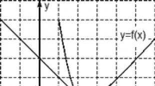
Task. The figure shows a graph of the function y = f(x) and a tangent to it at the point with the abscissa x 0. Find the value of the derivative of the function f(x) at the point x 0 .

Consider points A (0; 3) and B (3; 0), find the increments:
Δx = x 2 − x 1 = 3 − 0 = 3; Δy = y 2 − y 1 = 0 − 3 = −3.
Now we find the value of the derivative: D = Δy/Δx = −3/3 = −1.
Task. The figure shows a graph of the function y = f(x) and a tangent to it at the point with the abscissa x 0. Find the value of the derivative of the function f(x) at the point x 0 .

Consider points A (0; 2) and B (5; 2) and find the increments:
Δx = x 2 − x 1 = 5 − 0 = 5; Δy = y 2 − y 1 = 2 − 2 = 0.
It remains to find the value of the derivative: D = Δy/Δx = 0/5 = 0.
From the last example, we can formulate a rule: if the tangent is parallel to the OX axis, the derivative of the function at the point of tangency is zero. In this case, you don’t even need to count anything - just look at the graph.
Calculation of maximum and minimum points
Sometimes, instead of a graph of a function, Problem B9 gives a graph of the derivative and requires finding the maximum or minimum point of the function. In this situation, the two-point method is useless, but there is another, even simpler algorithm. First, let's define the terminology:
- The point x 0 is called the maximum point of the function f(x) if in some neighborhood of this point the following inequality holds: f(x 0) ≥ f(x).
- The point x 0 is called the minimum point of the function f(x) if in some neighborhood of this point the following inequality holds: f(x 0) ≤ f(x).
In order to find the maximum and minimum points from the derivative graph, just follow these steps:
- Redraw the derivative graph, removing all unnecessary information. As practice shows, unnecessary data only interferes with the decision. Therefore, we mark the zeros of the derivative on the coordinate axis - and that’s it.
- Find out the signs of the derivative on the intervals between zeros. If for some point x 0 it is known that f'(x 0) ≠ 0, then only two options are possible: f'(x 0) ≥ 0 or f'(x 0) ≤ 0. The sign of the derivative is easy to determine from the original drawing: if the derivative graph lies above the OX axis, then f'(x) ≥ 0. And vice versa, if the derivative graph lies below the OX axis, then f'(x) ≤ 0.
- We check the zeros and signs of the derivative again. Where the sign changes from minus to plus is the minimum point. Conversely, if the sign of the derivative changes from plus to minus, this is the maximum point. Counting is always done from left to right.
This scheme only works for continuous functions - there are no others in Problem B9.
Task. The figure shows a graph of the derivative of the function f(x) defined on the interval [−5; 5]. Find the minimum point of the function f(x) on this segment.

Let's get rid of unnecessary information and leave only the boundaries [−5; 5] and zeros of the derivative x = −3 and x = 2.5. We also note the signs:
Obviously, at the point x = −3 the sign of the derivative changes from minus to plus. This is the minimum point.
Task. The figure shows a graph of the derivative of the function f(x) defined on the interval [−3; 7]. Find the maximum point of the function f(x) on this segment.

Let's redraw the graph, leaving only the boundaries [−3; 7] and zeros of the derivative x = −1.7 and x = 5. Let us note the signs of the derivative on the resulting graph. We have:
![]()
Obviously, at the point x = 5 the sign of the derivative changes from plus to minus - this is the maximum point.
Task. The figure shows a graph of the derivative of the function f(x), defined on the interval [−6; 4]. Find the number of maximum points of the function f(x) belonging to the segment [−4; 3].

From the conditions of the problem it follows that it is enough to consider only the part of the graph limited by the segment [−4; 3]. Therefore, we build a new graph on which we mark only the boundaries [−4; 3] and zeros of the derivative inside it. Namely, points x = −3.5 and x = 2. We get:
![]()
On this graph there is only one maximum point x = 2. It is at this point that the sign of the derivative changes from plus to minus.
A small note about points with non-integer coordinates. For example, in the last problem the point x = −3.5 was considered, but with the same success we can take x = −3.4. If the problem is compiled correctly, such changes should not affect the answer, since the points “without a fixed place of residence” do not directly participate in solving the problem. Of course, this trick won’t work with integer points.
Finding intervals of increasing and decreasing functions
In such a problem, like the maximum and minimum points, it is proposed to use the derivative graph to find areas in which the function itself increases or decreases. First, let's define what increasing and decreasing are:
- A function f(x) is said to be increasing on a segment if for any two points x 1 and x 2 from this segment the following statement is true: x 1 ≤ x 2 ⇒ f(x 1) ≤ f(x 2). In other words, the larger the argument value, the larger the function value.
- A function f(x) is said to be decreasing on a segment if for any two points x 1 and x 2 from this segment the following statement is true: x 1 ≤ x 2 ⇒ f(x 1) ≥ f(x 2). Those. A larger argument value corresponds to a smaller function value.
Let us formulate sufficient conditions for increasing and decreasing:
- In order for a continuous function f(x) to increase on the segment , it is sufficient that its derivative inside the segment be positive, i.e. f’(x) ≥ 0.
- In order for a continuous function f(x) to decrease on the segment , it is sufficient that its derivative inside the segment be negative, i.e. f’(x) ≤ 0.
Let us accept these statements without evidence. Thus, we obtain a scheme for finding intervals of increasing and decreasing, which is in many ways similar to the algorithm for calculating extremum points:
- Remove all unnecessary information. In the original graph of the derivative, we are primarily interested in the zeros of the function, so we will leave only them.
- Mark the signs of the derivative at the intervals between zeros. Where f’(x) ≥ 0, the function increases, and where f’(x) ≤ 0, it decreases. If the problem sets restrictions on the variable x, we additionally mark them on a new graph.
- Now that we know the behavior of the function and the constraints, it remains to calculate the quantity required in the problem.
Task. The figure shows a graph of the derivative of the function f(x) defined on the interval [−3; 7.5]. Find the intervals of decrease of the function f(x). In your answer, indicate the sum of the integers included in these intervals.

As usual, let's redraw the graph and mark the boundaries [−3; 7.5], as well as zeros of the derivative x = −1.5 and x = 5.3. Then we note the signs of the derivative. We have:
![]()
Since the derivative is negative on the interval (− 1.5), this is the interval of decreasing function. It remains to sum all the integers that are inside this interval:
−1 + 0 + 1 + 2 + 3 + 4 + 5 = 14.
Task. The figure shows a graph of the derivative of the function f(x), defined on the interval [−10; 4]. Find the intervals of increase of the function f(x). In your answer, indicate the length of the largest of them.

Let's get rid of unnecessary information. Let us leave only the boundaries [−10; 4] and zeros of the derivative, of which there were four this time: x = −8, x = −6, x = −3 and x = 2. Let’s mark the signs of the derivative and get the following picture:
We are interested in the intervals of increasing function, i.e. such where f’(x) ≥ 0. There are two such intervals on the graph: (−8; −6) and (−3; 2). Let's calculate their lengths:
l 1 = − 6 − (−8) = 2;
l 2 = 2 − (−3) = 5.
Since we need to find the length of the largest of the intervals, we write down the value l 2 = 5 as an answer.
Let the function be defined at a point and some of its neighborhood. Let's give the argument an increment such that the point falls within the domain of definition of the function. The function will then be incremented.
DEFINITION. Derivative of a function at a point is called the limit of the ratio of the increment of the function at this point to the increment of the argument, at (if this limit exists and is finite), i.e.
Denote: ,,,.
Derivative of a function at a point on the right (left) called
(if this limit exists and is finite).
Designated by: , – derivative at the point on the right,
, is the derivative at the point on the left.
Obviously, the following theorem is true.
THEOREM. A function has a derivative at a point if and only if at this point the derivatives of the function on the right and left exist and are equal to each other. Moreover
The following theorem establishes a connection between the existence of a derivative of a function at a point and the continuity of the function at that point.
THEOREM (a necessary condition for the existence of a derivative of a function at a point). If a function has a derivative at a point, then the function at that point is continuous.
PROOF
Let it exist. Then
![]() ,
,
where is infinitesimal at.
Comment
derivative of a function and denote
differentiation of function .
GEOMETRICAL AND PHYSICAL MEANING
1) Physical meaning of the derivative. If a function and its argument are physical quantities, then the derivative is the rate of change of a variable relative to the variable at a point. For example, if is the distance traveled by a point in time, then its derivative is the speed at the moment of time. If is the amount of electricity flowing through the cross section of the conductor at an instant of time, then is the rate of change in the amount of electricity at an instant of time, i.e. current strength at a moment in time.
2) Geometric meaning of derivative.
Let be some curve, be a point on the curve. 
Any straight line intersecting at least two points is called secant .
Tangent to a curve at a point called the limit position of a secant if the point tends to, moving along a curve.
From the definition it is obvious that if a tangent to a curve exists at a point, then it is the only one
Consider a curve (i.e. a graph of a function). Let it have a non-vertical tangent at a point. Its equation: (equation of a straight line passing through a point and having an angular coefficient). 
By definition of the slope
where is the angle of inclination of the straight line to the axis.
Let be the angle of inclination of the secant to the axis, where. Since is a tangent, then when
Hence,
Thus, we got that – angular coefficient of the tangent to the graph of the function at the point(geometric meaning of the derivative of a function at a point). Therefore, the equation of the tangent to the curve at a point can be written in the form
Comment . A straight line passing through a point perpendicular to the tangent drawn to the curve at the point is called normal to the curve at the point . Since the angular coefficients of perpendicular straight lines are related by the relation, the equation of the normal to the curve at a point will have the form
![]() , If .
, If .
If , then the tangent to the curve at the point will have the form
and normal.
TANGENT AND NORMAL EQUATIONS
Tangent equation
Let the function be given by the equation y=f(x), you need to write the equation tangent at the point x 0. From the definition of derivative:
y/(x)=limΔ x→0Δ yΔ x
Δ y=f(x+Δ x)−f(x).
The equation tangent to the function graph: y=kx+b (k,b=const). From the geometric meaning of the derivative: f/(x 0)=tgα= k Because x 0 and f(x 0)∈ straight line, then the equation tangent is written as: y−f(x 0)=f/(x 0)(x−x 0) , or
y=f/(x 0)· x+f(x 0)−f/(x 0)· x 0.

Normal equation
Normal- is perpendicular to tangent(see picture). Based on this:
tgβ= tg(2π−α)= ctgα=1 tgα=1 f/(x 0)
Because the angle of inclination of the normal is angle β1, then we have:
tgβ1= tg(π−β)=− tgβ=−1 f/(x).
Dot ( x 0,f(x 0))∈ normal, the equation takes the form:
y−f(x 0)=−1f/(x 0)(x−x 0).
PROOF
Let it exist. Then
![]() ,
,
where is infinitesimal at.
But this means that it is continuous at a point (see the geometric definition of continuity). ∎
Comment . The continuity of a function at a point is not a sufficient condition for the existence of a derivative of this function at a point. For example, a function is continuous, but has no derivative at a point. Really,
and therefore does not exist.
Obviously, correspondence is a function defined on some set. They call her derivative of a function and denote
The operation of finding for a function its derivative function is called differentiation of function .
Derivative of sum and difference
Let functions f(x) and g(x) be given whose derivatives are known to us. For example, you can take the elementary functions discussed above. Then you can find the derivative of the sum and difference of these functions:
(f + g)’ = f ’ + g ’
(f − g)’ = f ’ − g ’
So, the derivative of the sum (difference) of two functions is equal to the sum (difference) of the derivatives. There may be more terms. For example, (f + g + h)’ = f’ + g’ + h’.
Strictly speaking, there is no concept of “subtraction” in algebra. There is a concept of “negative element”. Therefore, the difference f − g can be rewritten as the sum f + (−1) g, and then only one formula remains - the derivative of the sum.
The content of the article
DERIVATIVE– derivative of the function y = f(x), given on a certain interval ( a, b) at point x of this interval is called the limit to which the ratio of the increment of the function tends f at this point to the corresponding increment of the argument when the increment of the argument tends to zero.
The derivative is usually denoted as follows:
Other designations are also widely used:
Instant speed.
Let the point M moves in a straight line. Distance s moving point, counted from some initial position M 0 , depends on time t, i.e. s there is a function of time t: s= f(t). Let at some point in time t moving point M was at a distance s from the starting position M 0, and at some next moment t+D t found herself in a position M 1 - on distance s+D s from the initial position ( see pic.).
Thus, over a period of time D t distance s changed by the amount D s. In this case they say that during the time interval D t magnitude s received increment D s.
The average speed cannot in all cases accurately characterize the speed of movement of a point M at a point in time t. If, for example, the body at the beginning of the interval D t moved very quickly, and at the end very slowly, then the average speed will not be able to reflect the indicated features of the point’s movement and give an idea of the true speed of its movement at the moment t. To more accurately express the true speed using the average speed, you need to take a shorter period of time D t. Most fully characterizes the speed of movement of a point at the moment t the limit to which the average speed tends at D t® 0. This limit is called the current speed:
Thus, the speed of movement at a given moment is called the limit of the path increment ratio D s to time increment D t, when the time increment tends to zero. Because
Geometric meaning of the derivative. Tangent to the graph of a function.
The construction of tangent lines is one of those problems that led to the birth of differential calculus. The first published work related to differential calculus, written by Leibniz, was entitled A new method of maxima and minima, as well as tangents, for which neither fractional nor irrational quantities are an obstacle, and a special type of calculus for this.
Let the curve be the graph of the function y =f(x) in a rectangular coordinate system ( cm. rice.).
At some value x function matters y =f(x). These values x And y the point on the curve corresponds M 0(x, y). If the argument x give increment D x, then the new value of the argument x+D x corresponds to the new function value y+ D y = f(x + D x). The corresponding point of the curve will be the point M 1(x+D x,y+D y). If you draw a secant M 0M 1 and denoted by j the angle formed by a transversal with the positive direction of the axis Ox, it is immediately clear from the figure that .
If now D x tends to zero, then the point M 1 moves along the curve, approaching the point M 0, and angle j changes with D x. At Dx® 0 the angle j tends to a certain limit a and the straight line passing through the point M 0 and the component with the positive direction of the x-axis, angle a, will be the desired tangent. Its slope is:
Hence, f´( x) = tga
those. derivative value f´( x) for a given argument value x equals the tangent of the angle formed by the tangent to the graph of the function f(x) at the corresponding point M 0(x,y) with positive axis direction Ox.
Differentiability of functions.
Definition. If the function y = f(x) has a derivative at the point x = x 0, then the function is differentiable at this point.
Continuity of a function having a derivative. Theorem.
If the function y = f(x) is differentiable at some point x = x 0, then it is continuous at this point.
Thus, the function cannot have a derivative at discontinuity points. The opposite conclusion is incorrect, i.e. from the fact that at some point x = x 0 function y = f(x) is continuous does not mean that it is differentiable at this point. For example, the function y = |x| continuous for everyone x(–Ґ x x = 0 has no derivative. At this point there is no tangent to the graph. There is a right tangent and a left one, but they do not coincide.
Some theorems on differentiable functions. Theorem on the roots of the derivative (Rolle's theorem). If the function f(x) is continuous on the segment [a,b], is differentiable at all interior points of this segment and at the ends x = a And x = b goes to zero ( f(a) = f(b) = 0), then inside the segment [ a,b] there is at least one point x= With, a c b, in which the derivative fў( x) goes to zero, i.e. fў( c) = 0.
Finite increment theorem (Lagrange's theorem). If the function f(x) is continuous on the interval [ a, b] and is differentiable at all interior points of this segment, then inside the segment [ a, b] there is at least one point With, a c b that
f(b) – f(a) = fў( c)(b– a).
Theorem on the ratio of the increments of two functions (Cauchy's theorem). If f(x) And g(x) – two functions continuous on the segment [a, b] and differentiable at all interior points of this segment, and gў( x) does not vanish anywhere inside this segment, then inside the segment [ a, b] there is such a point x = With, a c b that
Derivatives of various orders.
Let the function y =f(x) is differentiable on some interval [ a, b]. Derivative values f ў( x), generally speaking, depend on x, i.e. derivative f ў( x) is also a function of x. When differentiating this function, we obtain the so-called second derivative of the function f(x), which is denoted f ўў ( x).
Derivative n- th order of function f(x) is called the (first order) derivative of the derivative n- 1- th and is denoted by the symbol y(n) = (y(n– 1))ў.
Differentials of various orders.
Function differential y = f(x), Where x– independent variable, yes dy = f ў( x)dx, some function from x, but from x only the first factor can depend f ў( x), the second factor ( dx) is the increment of the independent variable x and does not depend on the value of this variable. Because dy there is a function from x, then we can determine the differential of this function. The differential of the differential of a function is called the second differential or second-order differential of this function and is denoted d 2y:
d(dx) = d 2y = f ўў( x)(dx) 2 .
Differential n- of the first order is called the first differential of the differential n- 1- th order:
d n y = d(d n–1y) = f(n)(x)dx(n).
Partial derivative.
If a function depends not on one, but on several arguments x i(i varies from 1 to n,i= 1, 2,… n),f(x 1,x 2,… x n), then in differential calculus the concept of partial derivative is introduced, which characterizes the rate of change of a function of several variables when only one argument changes, for example, x i. 1st order partial derivative with respect to x i is defined as an ordinary derivative, and it is assumed that all arguments except x i, keep constant values. For partial derivatives, the notation is introduced
The 1st order partial derivatives defined in this way (as functions of the same arguments) can, in turn, also have partial derivatives, these are second order partial derivatives, etc. Such derivatives taken from different arguments are called mixed. Continuous mixed derivatives of the same order do not depend on the order of differentiation and are equal to each other.
Anna Chugainova
(\large\bf Derivative of a function)
Consider the function y=f(x), specified on the interval (a, b). Let x- any fixed point of the interval (a, b), A Δx- an arbitrary number such that the value x+Δx also belongs to the interval (a, b). This number Δx called argument increment.
Definition. Function increment y=f(x) at the point x, corresponding to the argument increment Δx, let's call the number
Δy = f(x+Δx) - f(x).
We believe that Δx ≠ 0. Consider at a given fixed point x the ratio of the function increment at this point to the corresponding argument increment Δx
We will call this relation the difference relation. Since the value x we consider fixed, the difference ratio is a function of the argument Δx. This function is defined for all argument values Δx, belonging to some sufficiently small neighborhood of the point Δx=0, except for the point itself Δx=0. Thus, we have the right to consider the question of the existence of a limit of the specified function at Δx → 0.
Definition. Derivative of a function y=f(x) at a given fixed point x called the limit at Δx → 0 difference ratio, that is
Provided that this limit exists.
Designation. y′(x) or f′(x).
Geometric meaning of derivative: Derivative of a function f(x) at this point x equal to the tangent of the angle between the axis Ox and a tangent to the graph of this function at the corresponding point:
f′(x 0) = \tgα.
Mechanical meaning of derivative: The derivative of the path with respect to time is equal to the speed of rectilinear motion of the point:
Equation of a tangent to a line y=f(x) at the point M 0 (x 0 ,y 0) takes the form
y-y 0 = f′(x 0) (x-x 0).
The normal to a curve at some point is the perpendicular to the tangent at the same point. If f′(x 0)≠ 0, then the equation of the normal to the line y=f(x) at the point M 0 (x 0 ,y 0) is written like this:

The concept of differentiability of a function
Let the function y=f(x) defined over a certain interval (a, b), x- some fixed argument value from this interval, Δx- any increment of the argument such that the value of the argument x+Δx ∈ (a, b).
Definition. Function y=f(x) called differentiable at a given point x, if increment Δy this function at the point x, corresponding to the argument increment Δx, can be represented in the form
Δy = A Δx +αΔx,
Where A- some number independent of Δx, A α - argument function Δx, which is infinitesimal at Δx→ 0.
Since the product of two infinitesimal functions αΔx is an infinitesimal of a higher order than Δx(property of 3 infinitesimal functions), then we can write:
Δy = A Δx +o(Δx).
Theorem. In order for the function y=f(x) was differentiable at a given point x, it is necessary and sufficient that it has a finite derivative at this point. Wherein A=f′(x), that is
Δy = f′(x) Δx +o(Δx).
The operation of finding the derivative is usually called differentiation.
Theorem. If the function y=f(x) x, then it is continuous at this point.
Comment. From the continuity of the function y=f(x) at this point x, generally speaking, the differentiability of the function does not follow f(x) at this point. For example, the function y=|x|- continuous at a point x=0, but has no derivative.
Concept of differential function
Definition. Function differential y=f(x) the product of the derivative of this function and the increment of the independent variable is called x:
dy = y′ Δx, df(x) = f′(x) Δx.
For function y=x we get dy=dx=x′Δx = 1· Δx= Δx, that is dx=Δx- the differential of an independent variable is equal to the increment of this variable.
Thus, we can write
dy = y′ dx, df(x) = f′(x) dx
![]()
Differential dy and increment Δy functions y=f(x) at this point x, both corresponding to the same argument increment Δx, generally speaking, are not equal to each other.
Geometric meaning of differential: The differential of a function is equal to the increment of the ordinate of the tangent to the graph of this function when the argument is incremented Δx.
Rules of differentiation
Theorem. If each of the functions u(x) And v(x) differentiable at a given point x, then the sum, difference, product and quotient of these functions (quotient provided that v(x)≠ 0) are also differentiable at this point, and the formulas hold:

Consider the complex function y=f(φ(x))≡ F(x), Where y=f(u), u=φ(x). In this case u called intermediate argument, x - independent variable.
Theorem. If y=f(u) And u=φ(x) are differentiable functions of their arguments, then the derivative of a complex function y=f(φ(x)) exists and is equal to the product of this function with respect to the intermediate argument and the derivative of the intermediate argument with respect to the independent variable, i.e.
![]()
Comment. For a complex function that is a superposition of three functions y=F(f(φ(x))), the differentiation rule has the form
y′ x = y′ u u′ v v′ x,
where are the functions v=φ(x), u=f(v) And y=F(u)- differentiable functions of their arguments.
Theorem. Let the function y=f(x) increases (or decreases) and is continuous in some neighborhood of the point x 0. Let, in addition, this function be differentiable at the indicated point x 0 and its derivative at this point f′(x 0) ≠ 0. Then in some neighborhood of the corresponding point y 0 =f(x 0) the inverse is defined for y=f(x) function x=f -1 (y), and the indicated inverse function is differentiable at the corresponding point y 0 =f(x 0) and for its derivative at this point y the formula is valid

Derivatives table

Invariance of the form of the first differential
Let's consider the differential of a complex function. If y=f(x), x=φ(t)- functions of their arguments are differentiable, then the derivative of the function y=f(φ(t)) expressed by the formula
y′ t = y′ x x′ t.
A-priory dy=y′ t dt, then we get
dy = y′ t dt = y′ x · x′ t dt = y′ x (x′ t dt) = y′ x dx,
dy = y′ x dx.
So, we have proven
Property of invariance of the form of the first differential of a function: as in the case when the argument x is an independent variable, and in the case when the argument x itself is a differentiable function of the new variable, the differential dy functions y=f(x) is equal to the derivative of this function multiplied by the differential of the argument dx.
Application of differential in approximate calculations
We have shown that the differential dy functions y=f(x), generally speaking, is not equal to the increment Δy this function. However, up to an infinitesimal function of a higher order of smallness than Δx, the approximate equality is valid
Δy ≈ dy.
The ratio is called the relative error of the equality of this equality. Because Δy-dy=o(Δx), then the relative error of this equality becomes as small as desired with decreasing |Δх|.
Considering that Δy=f(x+δ x)-f(x), dy=f′(x)Δx, we get f(x+δ x)-f(x) ≈ f′(x)Δx or
f(x+δ x) ≈ f(x) + f′(x)Δx.
This approximate equality allows with error o(Δx) replace function f(x) in a small neighborhood of the point x(i.e. for small values Δx) linear function of the argument Δx, standing on the right side.
Higher order derivatives
Definition. Second derivative (or second order derivative) of a function y=f(x) is called the derivative of its first derivative.
Notation for the second derivative of a function y=f(x):
Mechanical meaning of the second derivative. If the function y=f(x) describes the law of motion of a material point in a straight line, then the second derivative f″(x) equal to the acceleration of a moving point at the moment of time x.
The third and fourth derivatives are determined similarly.
Definition. n th derivative (or derivative n-th order) functions y=f(x) is called the derivative of it n-1 th derivative:
y (n) =(y (n-1))′, f (n) (x)=(f (n-1) (x))′.
Designations: y″′, y IV, y V etc.
Geometric meaning of derivative
|
DEFINITION OF TANGENT TO A CURVE Tangent to a curve y=ƒ(x) at the point M is called the limiting position of a secant drawn through a point M and the point adjacent to it M 1 curve, provided that the point M 1 approaches indefinitely along the curve to the point M. GEOMETRICAL MEANING OF DERIVATIVE Derivative of a function y=ƒ(x) at the point X 0 is numerically equal to the tangent of the angle of inclination to the axis Oh tangent to the curve y=ƒ(x) at the point M (x 0; ƒ(x 0)). |
VARIATION DOTIC TO CURVE Dotted to the curve y=ƒ(x) exactly M is called the boundary position of the line drawn through the point M and the next point with her M 1 crooked, beyond the mind, what a point M 1 the curve is inevitably approaching the point M. GEOMETRICAL ZMIST POKHIDNOI Similar functions y=ƒ(x) exactly x 0 numerically equal to the tangent of the slope to the axis Oh dotic, carried out to the curve y=ƒ(x) exactly M (x 0; ƒ(x 0)). |
Practical meaning of derivative
Let's consider what the quantity we found as a derivative of a certain function practically means.
First of all, derivative- this is the basic concept of differential calculus, characterizing the rate of change of a function at a given point.
What is "rate of change"? Let's imagine the function f(x) = 5. Regardless of the value of the argument (x), its value does not change in any way. That is, the rate of its change is zero.
Now consider the function f(x) = x. The derivative of x is equal to one. Indeed, it is easy to notice that for every change in the argument (x) by one, the value of the function also increases by one.
From the point of view of the information received, now let's look at the table of derivatives of simple functions. Based on this, the physical meaning of finding the derivative of a function immediately becomes clear. This understanding should make it easier to solve practical problems.
Accordingly, if the derivative shows the rate of change of a function, then the double derivative shows acceleration.
2080.1947