Fairy tales

Measuring technology. Determination of electromotive force and specific thermo-emf of a thermocouple

9.1. Goal of the work

Determination of the dependence of the thermoelectromotive force of a thermocouple on the temperature difference between the junctions.

In a closed circuit (Fig. 9.1), consisting of dissimilar conductors (or semiconductors) A and B, an electromotive force (emf) E T arises and a current flows if contacts 1 and 2 of these conductors are maintained at different temperatures T 1 and T 2. This e.m.f. is called thermoelectromotive force (thermo-emf), and an electrical circuit of two dissimilar conductors is called a thermocouple. When the sign of the junction temperature difference changes, the direction of the thermocouple current changes. This
the phenomenon is called the Seebeck phenomenon.

There are three known reasons for the occurrence of thermo-EMF: the formation of a directed flow of charge carriers in a conductor in the presence of a temperature gradient, the entrainment of electrons by phonons, and a change in the position of the Fermi level depending on temperature. Let's look at these reasons in more detail.

In the presence of a temperature gradient dT / dl along the conductor, electrons at its hot end have greater kinetic energy, and therefore a greater speed of chaotic movement compared to electrons at the cold end. As a result, a preferential flow of electrons occurs from the hot end of the conductor to the cold one, a negative charge accumulates at the cold end, and an uncompensated positive charge remains at the hot end.

The accumulation continues until the resulting potential difference causes an equal flow of electrons. The algebraic sum of such potential differences in the circuit creates the volumetric component of the thermo-emf.

In addition, the existing temperature gradient in the conductor leads to the emergence of a preferential movement (drift) of phonons (quanta of vibrational energy of the crystal lattice of the conductor) from the hot end to the cold end. The existence of such a drift leads to the fact that electrons scattered by phonons themselves begin to make a directed movement from the hot end to the cold one. The accumulation of electrons at the cold end of the conductor and the depletion of electrons at the hot end leads to the appearance of a phonon component of the thermo-emf. Moreover, at low temperatures, the contribution of this component is the main one in the occurrence of thermal emf.

As a result of both processes, an electric field appears inside the conductor, directed towards the temperature gradient. The strength of this field can be represented as

E = -dφ / dl = (-dφ / dT)· (-dt / dl)=-β·(-dT / dl)

where β = dφ / dT.

Relation (9.1) connects the electric field strength E with the temperature gradient dT / dl. The resulting field and temperature gradient have opposite directions, so they have different signs.

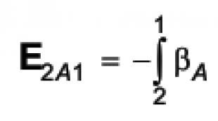
The field defined by expression (9.1) is the field of external forces. Having integrated the strength of this field over the section of circuit AB (Figure 9.1) from junction 2 to junction 1 and assuming that T 2 > T 1, we obtain an expression for the thermal emf acting in this section:

(The sign changed when the integration limits changed.) Similarly, we determine the thermal emf acting in section B from junction 1 to junction 2.

The third reason for the occurrence of thermo-emf. depends on the temperature of the position of the Fermi level, which corresponds to the highest energy level occupied by electrons. The Fermi level corresponds to the Fermi energy E F that electrons can have at this level.

Fermi energy is the maximum energy that conduction electrons in a metal can have at 0 K. The higher the density of the electron gas, the higher the Fermi level will be. For example (Fig. 9.2), E FA is the Fermi energy for metal A, and E FB for metal B. The values of E PA and E PB are the highest potential energy of electrons in metals A and B, respectively. When two dissimilar metals A and B come into contact, the presence of a difference in Fermi levels (E FA > E FB) leads to the occurrence of a transition of electrons from metal A (with a higher level) to metal B (with a low Fermi level).

In this case, metal A becomes positively charged, and metal B negatively. The appearance of these charges causes a shift in the energy levels of metals, including Fermi levels. As soon as the Fermi levels are equalized, the reason causing the preferential transfer of electrons from metal A to metal B disappears, and a dynamic equilibrium is established between the metals. From Fig. 9.2 it is clear that the potential energy of an electron in metal A is less than in B by the amount E FA - E FB. Accordingly, the potential inside metal A is higher than inside B by the amount)

U AB = (E FA - E FB) / l

This expression gives the internal contact potential difference. The potential decreases by this amount during the transition from metal A to metal B. If both thermocouple junctions (see Fig. 9.1) are at the same temperature, then the contact potential differences are equal and directed in opposite directions.

In this case they compensate each other. It is known that the Fermi level, although weakly, depends on temperature. Therefore, if the temperatures of junctions 1 and 2 are different, then the difference U AB (T 1) - U AB (T 2) at the contacts makes its contact contribution to the thermo-emf. It can be comparable to volumetric thermal emf. and is equal to:

E contact = U AB (T 1) - U AB (T 2) = (1/l) · ( + )

The last expression can be represented as follows:

The resulting thermal emf. (ε T) consists of the emf acting in contacts 1 and 2 and the emf acting in sections A and B.

E T = E 2A1 + E 1B2 + E contact

Substituting expressions, (9.3) and (9.6) into (9.7) and carrying out transformations, we obtain

where α = β - ((1/l) (dE F / dT))

The quantity α is called the thermo-emf coefficient. Since both β and dE F / d T depend on temperature, the coefficient α is also a function of T.

Taking into account (9.9), the expression for thermo-emf can be presented as:

The quantity α AB is called differential or at effective thermo-EMF given pair of metals. It is measured in V/K and significantly depends on the nature of the contacting materials, as well as the temperature range, reaching about 10 -5 ÷10 -4 V/K. In a small temperature range (0-100°C), the specific thermal emf. weakly depends on temperature. Then formula (9.11) can be represented with a sufficient degree of accuracy in the form:

E T = α (T 2 - T 1)

In semiconductors, unlike metals, there is a strong dependence of the concentration of charge carriers and their mobility on temperature. Therefore, the effects discussed above, leading to the formation of thermal emf, are more pronounced in semiconductors, the specific thermal emf. much larger and reaches values of the order of 10 -3 V/K.

9.3. Description of the laboratory setup

To study the dependence of thermo-emf. on the temperature difference between the junctions (contacts), in this work we use a thermocouple made of two pieces of wire, one of which is a chromium-based alloy (chromel), and the other an aluminum-based alloy (alumel). One junction together with a thermometer is placed in a vessel with water, the temperature T 2 of which can be changed by heating on an electric stove. The temperature of the other junction T 1 is maintained constant (Fig. 9.3). The resulting thermal emf. measured with a digital voltmeter.

9.4. Experimental procedure and results processing
9.4.1. Experimental technique

The work uses direct measurements of the emf generated in the thermocouple. The temperature of the junctions is determined by the temperature of the water in the vessels using a thermometer (see Fig. 9.3)

9.4.2. Work order

Plug in the voltmeter's power cord.
Press the power button on the front panel of the digital voltmeter. Let the device warm up for 20 minutes.
Loosen the clamp screw on the thermocouple stand, lift it up and secure it. Pour cold water into both glasses. Drop the thermocouple junctions into the glasses to approximately half the depth of the water.
Write it down in the table. 9.1 the value of the initial temperature T 1 of the junctions (water) according to the thermometer (for the other junction it remains constant throughout the experiment).
Turn on the electric stove.
Record the emf values. and temperatures T 2 in table. 9.1 every ten degrees.
When the water boils, turn off the electric stove and voltmeter.

9.4.3. Processing of measurement results

Based on the measurement data, construct a graph of the emf. thermocouples 8T (ordinate axis) from the temperature difference between the junctions ΔT = T 2 - T 1 (abscissa axis).
Using the resulting graph of the linear dependence of E T on ∆T, determine the specific thermal emf. according to the formula: α = ΔE T / Δ(ΔT)

9.5. Checklist

What is the essence and what is the nature of the Seebeck phenomenon?
What causes the appearance of the volumetric component of thermo-emf?
What causes the appearance of the phonon component of the thermo-emf?
What causes the occurrence of a contact potential difference?
What devices are called thermocouples and where are they used?
What is the essence and what is the nature of the Peltier and Thomson phenomena?

Savelyev I.V. Course of general physics. T.3. - M.: Nauka, 1982. -304 p.
Epifanov G.I. Solid State Physics. M.: Higher School, 1977. - 288 p.
Sivukhin D.V. General course in physics. Electricity. T.3. - M.: Nauka, 1983. -688 p.
Trofimova T.I. Physics course. M.: Higher School, 1985. - 432 p.
Detlaf A. A., Yavorsky V. M. Physics course. M.: Higher School, 1989. - 608 p.

Thermoelectric converters. Operating principle, materials used.

A thermal converter is a converter whose operating principle is based on thermal processes and whose natural input quantity is temperature. Such converters include thermocouples and thermistors, metal and semiconductor. The main equation of thermal conversion is the heat balance equation, the physical meaning of which is that all the heat supplied to the converter goes to increase its heat content QTC and, therefore, if the heat content of the converter remains unchanged (the temperature and state of aggregation do not change), then the quantity The amount of heat received per unit time is equal to the amount of heat given off. The heat supplied to the converter is the sum of the amount of heat Qel created as a result of the release of electrical power in it, and the amount of heat Qto entering the converter or given off by it as a result of heat exchange with the environment.

The phenomenon of thermoelectricity was discovered in 1823 by Seebeck and is as follows. If you make a circuit of two different conductors (or semiconductors) A and B, connecting them to each other at their ends (Fig. 1), and making the temperature 1 of one connection point different from the temperature 0 of the other, then an emf will appear in the circuit. , called thermoelectromotive force (thermo-emf) and representing the difference in functions of temperatures, junctions of conductors.

Such a circuit is called a thermoelectric converter or otherwise thermocouple; the conductors that make up the thermocouple are called thermoelectrodes, and their connections are called junctions.

Fig.1.

With a small temperature difference between the junctions, the thermo-emf. can be considered proportional to the temperature difference.

Experience shows that for any pair of homogeneous conductors that obey Ohm’s law, the magnitude of the thermo-emf. depends only on the nature of the conductors and on the temperature of the junctions and does not depend on the temperature distribution between the junctions.

The operation of a thermocouple is based on the Seebeck effect. The Seebeck effect is based on the following phenomena. If there is a temperature gradient along a conductor, the electrons at the hot end produce higher energies and velocities than those at the cold end. As a result, a flow of electrons occurs from the hot end to the cold end, and a negative charge accumulates at the cold end, and an uncompensated positive charge remains at the hot end. Since the average energy of electrons depends on the nature of the conductor and increases differently with temperature, for the same temperature difference the thermo-EMF at the ends of different conductors will be different:

E1 = k1(T1 - T2); e2 = k2(T1 - T2)

Where T1 and T2 are the temperatures of the hot and cold ends, respectively; k1 and k2 are coefficients that depend on the physical properties of the 1st and 2nd conductors, respectively. The resulting potential difference is called volumetric thermo-EPC:

Eob = e1 - e2 = (k1 - k2)(T1 - T2).

In places where dissimilar conductors are soldered, a contact potential difference appears, which depends on the area and materials of the adjacent surfaces and is proportional to their temperature:

Ek1 = kpovT1; ek2 = kpovT2

Where kpov is the coefficient of surfaces of tangent metals. As a result, the second component of the initial voltage appears - contact thermo-EPC:

Ek = ek1 - ek2 = ksur(T1 - T2)

The voltage at the thermocouple output is determined as the sum of volumetric and contact thermo-EMF:

Uin = erev + ek = (k1 - k2 + ksur)(T1 - T2) = k(T1 - T2)

Where k is the transmission coefficient.

Disadvantages of a thermocouple:

Low sensitivity (about 0.1 mV/°K);
- high initial resistance;
- the need to maintain a constant temperature of one of the ends.

The phenomenon of thermoelectricity is one of the reversible phenomena; the reverse effect was discovered in 1834 by Jean Peltier and named after him.
If an electric current is passed through a circuit consisting of two different conductors or semiconductors, heat is generated at one junction and absorbed at the other. Peltier heat is related to current strength in a linear relationship, unlike Joule heat, and depending on the direction of the current, the junction is heated or cooled.
The absorbed or released thermal power is proportional to the current strength, depends on the nature of the materials forming the junction, and is characterized by the Peltier coefficient.

Efficiency thermoelectric generator depends on the temperature difference and properties of materials and for existing materials is very small (at = 300° does not exceed = 13%, and at = 100° the value = 5%), therefore thermoelectric generators are used as energy generators only in special conditions. Efficiency thermoelectric heater and refrigerator are also very small, and the cooling efficiency is with a temperature difference of 5° it is 9%, and with a temperature difference of 40° - only 0.6%; however, despite such low efficiency, thermoelements are used in refrigeration devices. In measurement technology, thermocouples are widely used for measuring temperatures; In addition, semiconductor thermoelements are used as reverse thermal converters, converting electric current into heat flow and temperature.

A thermocouple with a millivoltmeter connected to it, used to measure temperature.
If one thermocouple junction, called the working junction, is placed in an environment with temperature 1 to be measured, and the temperature of the other 2, non-working junctions is kept constant, then f(0) = const and EAB(1) = f(1) – C= f1(1). regardless of how the thermoelectrodes are connected (soldering, welding, etc.). Thus, the natural input value of a thermocouple is the temperature of its working junction, and the output value is thermo-e. d.s., which the thermocouple develops at a strictly constant temperature of 2 non-working junctions.

Materials used for thermocouples. In table Figure 1 shows the thermo-emf that is developed by various thermoelectrodes paired with platinum at the temperature of the working junction 1 = 100°C and the temperature of the non-working junction 2 = 0°C. The dependence of the thermo-emf. on temperature over a wide temperature range is usually nonlinear, so the table data cannot be extended to higher temperatures.

Table 1.

Material	Thermo-emf, mV	Material	Thermo-emf, mV



		Aluminum


Molybdenum
		Palladium
Tungsten
Manganin

		Constantan


		Molybdenum

When using the table data, it should be borne in mind that the thermo-emf developed by thermoelectrodes. largely depend on the slightest impurities, mechanical processing (hardening) and heat treatment (hardening, annealing).

When designing thermocouples, one naturally strives to combine thermo-electrodes, one of which develops a positive thermo-emf with platinum, and the other a negative thermo-emf. In this case, it is also necessary to take into account the suitability of a particular thermoelectrode for use under the given measurement conditions (the influence of the environment, temperature, etc. on the thermoelectrode).
To increase the output emf. Several thermocouples are used to form a thermopile. The working junctions of thermocouples are located on a blackened lobe that absorbs radiation, the cold ends are located on a massive copper ring that serves as a heat sink and is covered with a screen. Due to the massiveness and good heat transfer of the ring, the temperature of the free ends can be considered constant and equal to room temperature.

Errors and corrections of thermocouple measurements.

A measuring device or electronic measuring system is connected either to the ends of the thermoelectrodes (Fig. 2, a) or to the gap of one of them (Fig. 2, b).

Fig.2 Connecting the measuring device to the thermocouple

Error caused by changes in the temperature of the non-working junctions of the thermocouple. Thermocouple calibration is carried out at the temperature of the non-working junctions equal to zero. If, during the practical use of a thermoelectric pyrometer, the temperature of the non-working junctions differs from 0 ° C by a value of 0, then it is necessary to introduce an appropriate correction to the thermometer readings.

However, it should be borne in mind that due to the nonlinear relationship between the emf. thermocouple and the temperature of the working junction, the amount of correction to the readings of the pointer, calibrated directly in degrees, will not be equal to the temperature difference 0 of the free ends.
The magnitude of the correction is related to the temperature difference between the free ends through a coefficient k called the correction factor for the temperature of the non-working ends. The value of k is different for each section of the curve, therefore the calibration curve is divided into sections of 100° C and the value of k is determined for each section.

The disadvantage of such devices is the need for a current source to power the bridge and the appearance of an additional error caused by changes in the voltage of this source.

Error due to changes in temperature of the line, thermocouple and pointer. In thermoelectric thermometers for measuring thermo-emf. Both conventional millivoltmeters and low-resistance compensators with manual or automatic balancing for a measurement limit of up to 100 mV are used.

In cases where the thermo-emf. is measured by a compensator, the resistance of the thermo-emf circuit, as is known, does not play a role. In the same cases when thermo-emf. measured with a millivoltmeter, an error may occur due to changes in the resistances of all elements that make up the thermo-emf circuit; therefore, it is necessary to strive for a constant resistance value of the wires and the thermocouple itself

Industrial thermocouples

Main parameters of industrial thermocouples:

table 2

Thermocouple designation	Designation of thermoelectrodes	Materials	Measurement limits for long-term use	Upper measurement limit for short-term use
		Platinorhodium (10% rhodium) platinum	From -20 to 1300
		Platinorhodium (30% rhodium)
		Chromel-alumel
		Chromel-kopel

To measure temperatures below - 50 ° C, special thermocouples can be used, for example, copper - constantan (up to ~ - 270 ° C), copper - copel (up to - 200 ° C), etc. For measuring temperatures above 1300-1800 ° Thermocouples are manufactured based on refractory metals: iridium-rhenium-iridium (up to 2100° C), tungsten-rhenium (up to 2500° C), based on transition metal carbides - titanium, zirconium, niobium, thalia, hafnium
(theoretically up to 3000-3500 ° C), based on carbon and graphite fibers.
The calibration characteristics of thermocouples of the main types are given in table. 3. This table shows the temperature of the working junction in degrees
Celsius and the values of thermo-emf are given. corresponding thermocouples in millivolts at a temperature of the free ends of 0 ° C.

Table 3

Graduation designation	Working junction temperature
	12.2, 16.40, 20.65, 24.91, 33.32, 41.26, 48.87
	2.31, 3.249, 4.128, 5.220, 7.325, 9.564, 11.92, 14.33, 16.71
	4.913, 6.902, 9.109, 11.47, 13.92

Deviations of real thermo-emf are allowed. from the values given in table. 3, by the values indicated in table. 4.

Table 4

Industrial Type Thermocouple Design. This is a thermocouple with thermoelectrodes made of base metals located in a composite protective tube with a movable flange for its fastening. The working junction of the thermocouple is insulated with a tip. The thermoelectrodes are insulated with bars. The protective pipe consists of a working and non-working section. The movable flange is attached to the pipe with a screw. The thermocouple head has a cast housing with a cover secured with screws; The head is reinforced with porcelain pads (screws) with floating (loose) clamps, which allow the thermoelectrodes to elongate under the influence of temperature without the occurrence of mechanical stresses leading to rapid destruction of the thermoelectrodes. The thermoelectrodes are attached to these clamps with screws, and the connecting wires are attached with screws. These wires pass through a fitting with an asbestos seal.

For noble metal thermocouples, non-metallic tubes (quartz, porcelain, etc.) are often used, but such tubes are mechanically fragile and expensive. Porcelain pipes of the proper composition can be used at temperatures up to 1300-1400°C.
Asbestos is used to insulate thermoelectrodes from each other up to 300°C, quartz tubes or beads up to 1000°C, porcelain pipes up to 1300C. For laboratory thermocouples used in measuring low temperatures, heat-resistant rubber is also used up to 150°C, silk up to 100 -120°C, enamel up to 150-200°C.

Methods of contact electrical measurements of medium and high temperatures using thermocouples

In thermometry, temperatures from 500 (beginning of glow) to 1600 °C (white heat) are considered average, and high temperatures are from 1600 to 2500 °C, to which it is possible to extend the thermoelectric method using high-temperature, heat-resistant materials.
The principle of the thermoelectric method and the basic properties of thermoelectrodes were discussed above in paragraph 1. The main issue when using this method to measure medium and high temperatures is the protection of thermoelectrodes from the destructive chemical and thermal effects of the environment. For this purpose, thermocouples are equipped with protective fittings in the form of covers, tubes or caps made of refractory materials. The main requirement for a protective shell is high structural density and temperature resistance.

When measuring temperatures below 1300 °C, porcelain covers are used, at higher temperatures - caps made of refractory materials (such as corundum, aluminum oxide, beryllium or thorium) filled with an inert gas.

Dependence of the service life of thermocouples on the porosity of the protective shell.

When measuring the surface temperature of bodies, a particular difficulty is the contact of the working junction of the thermocouple with the surface of the heated body.
To improve contact, thermocouples are used, the working junction of which is made in the form of a tape or plate. This configuration of the working junction during deformation makes it possible to reproduce the surface of the measurement object.

To measure temperatures up to 2000-2500 °C, tungsten or iridium thermocouples are used. A special feature of their use is measurement in a vacuum, in inert or reducing environments, since they oxidize in air. The sensitivity of a tungsten-molybdenum thermocouple is 7 μV/K, and a tungsten-rhenium thermocouple is 13 μV/K.
At high temperatures, thermocouples made of refractory materials are used (pairs of titanium carbide - graphite, zirconium carbide - zirconium boride and molybdenum disilicide - tungsten disilicide). In such thermocouples, inside a cylindrical electrode (diameter about 15 mm) there is a second rod electrode connected to the first electrode at one end of the tube.

The sensitivity of thermocouples made of refractory materials reaches 70 μV/K, but their use is limited to inert and reducing media.
To measure the temperature of molten metal with noble metal thermocouples, a method is used that involves immersing the thermocouple in the metal for a period of time that is safe for its operation. In this case, the thermocouple is immersed in a controlled environment for a short time (0.4-0.6 s), and the rate of increase in the temperature of the working junction is measured. Knowing the relationship between the heating rate of the thermocouple (its thermal inertia) and the temperature environment, you can calculate the value of the measured temperature. This method is used to measure molten metal (2000-2500 C) and gas flow (1800 C).

Thermocouple (thermoelectric converter) is a device used to measure temperature in industry, scientific research, medicine, and in automation systems.

The operating principle is based on the Seebeck effect or, in other words, the thermoelectric effect. There is a contact potential difference between the connected conductors; if the joints of conductors connected in a ring are at the same temperature, the sum of such potential differences is equal to zero. When the joints are at different temperatures, the potential difference between them depends on the temperature difference. The proportionality coefficient in this dependence is called the thermo-EMF coefficient. Different metals have different thermo-emf coefficients and, accordingly, the potential difference arising between the ends of different conductors will be different. By placing a junction of metals with non-zero thermo-emf coefficients in an environment with a temperature T 1, we get the voltage between opposite contacts located at a different temperature T 2, which will be proportional to the temperature difference T 1 and T 2 .

Advantages of thermocouples

High accuracy of temperature measurement (up to ±0.01 °C).
Large temperature measurement range: from −250 °C to +2500 °C.
Simplicity.
Cheapness.
Reliability

To obtain high accuracy of temperature measurement (up to ±0.01 °C), individual calibration of the thermocouple is required.
The readings are affected by the riser temperature, which must be corrected for. Modern thermocouple-based meter designs use the measurement of the cold junction block temperature using a built-in thermistor or semiconductor sensor and automatically correct for the measured emf.
Peltier effect (at the time of taking readings, it is necessary to exclude the flow of current through the thermocouple, since the current flowing through it cools the hot junction and heats up the cold one).
The dependence of TEMF on temperature is significantly nonlinear. This creates difficulties when developing secondary signal converters.
The occurrence of thermoelectric inhomogeneity as a result of sudden temperature changes, mechanical stresses, corrosion and chemical processes in conductors leads to changes in the calibration characteristics and errors of up to 5 K.
Over long lengths of thermocouple and extension wires, an “antenna” effect may occur to existing electromagnetic fields.

Technical requirements for thermocouples are determined by GOST 6616-94. Standard tables for thermoelectric thermometers (NSH), tolerance classes and measurement ranges are given in the IEC 60584-1.2 standard and GOST R 8.585-2001.

platinum-rhodium-platinum - TPP13 - Type R
platinum-rhodium-platinum - TPP10 - Type S
platinumrhodium-platinumrhodium - TPR - Type B
iron-constantan (iron-copper-nickel) TLC - Type J
copper-constantan (copper-copper-nickel) TMKn - Type T
nichrosil-nisil (nickel-chrome-nickel-nickel-silicon) TNN - Type N.
chromel-alumel - THA - Type K
chromel-constantan THCn - Type E
chromel-copel - THK - Type L
copper-copel - TMK - Type M
sil-silin - TCC - Type I
tungsten and rhenium - tungsten rhenium - TVR - Type A-1, A-2, A-3

To use the online calculator, in the “Thermo-EMF (mV)” field, you must enter the value of the thermo-EMF of the thermocouple; you should also take into account that the temperature will be displayed without taking into account the ambient temperature. For ease of use of the online calculator, in the “Ambient temperature” field. environment" you must enter the ambient temperature in °C and all readings will be with the ambient temperature leaked.

Online calculator converting thermo-EMF to temperature (°C) for a chromel-alumel thermocouple - TXA - Type K.

Online calculator

chromel-alumel type - TXA - Type K.

Online calculator converting thermo-EMF to temperature (°C) for a thermocouple type

chromel-copel - TXK - Type L.