Transformation of rectangular coordinates on the plane. Transformation of Cartesian rectangular coordinates on the plane and in space. I. Privalov "Analytical geometry"
Chapter I. Vectors on the plane and in space
§ 13. Transition from one rectangular Cartesian coordinate system to another
We offer you to consider this topic in two versions.
1) Based on the textbook by I.I. Privalov "Analytical Geometry" (textbook for higher technical educational institutions, 1966)
I.I. Privalov "Analytical geometry"
§ 1. The problem of coordinate transformation.
The position of a point on the plane is determined by two coordinates relative to some coordinate system. The coordinates of the point will change if we choose a different coordinate system.
The task of transforming coordinates is to to, knowing the coordinates of a point in one coordinate system, find its coordinates in another system.
This problem will be solved if we establish formulas that relate the coordinates of an arbitrary point in two systems, and the coefficients of these formulas will include constant values that determine the mutual position of the systems.
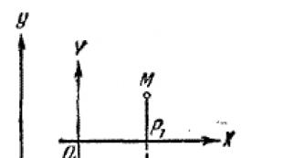
Let two Cartesian coordinate systems be given hoy And XO 1Y(Fig. 68).
Position of the new system XO 1Y relative to the old system hoy will be determined if the coordinates are known A And b new beginning O 1 according to the old system and the angle α between axles Oh And About 1 X. Denote by X And at coordinates of an arbitrary point M relative to the old system, through X and Y-coordinates of the same point relative to the new system. Our task is to make the old coordinates X And at expressed in terms of the new X and Y. The resulting transformation formulas must obviously include the constants a, b And α .
We will obtain the solution of this general problem by considering two particular cases.
1. The origin of coordinates changes, while the directions of the axes remain unchanged ( α = 0).
2. The directions of the axes change, while the origin of coordinates remains unchanged ( a = b = 0).
§ 2. Transfer of the origin.
Let two systems of Cartesian coordinates with different origins be given O And O 1 and the same directions of the axes (Fig. 69).

Denote by A And b coordinates of a new beginning About 1 in the old system and through x, y And X, Y-coordinates of an arbitrary point M, respectively, in the old and new systems. Projecting point M on the axis About 1 X And Oh, as well as the point About 1 per axle Oh, we get on the axis Oh three dots Oh, a And R. Segment values OA, AR And OR are related by the following relation:
| OA| + | AR | = | OR |. (1)
Noticing that | | OA| = A , | OR | = X , | AR | = | O 1 R 1 | = X, we rewrite equality (1) in the form:
A + X = x or x = X + A . (2)
Similarly, projecting M and About 1 on the y-axis, we get:
y = Y + b (3)
So, the old coordinate is equal to the new one plus the coordinate of the new origin according to the old system.
From formulas (2) and (3), the new coordinates can be expressed in terms of the old ones:
X = x - a , (2")
Y = y-b . (3")
§ 3. Rotation of the coordinate axes.
Let two Cartesian coordinate systems with the same origin be given ABOUT and different directions of the axes (Fig. 70).

Let α is the angle between the axes Oh And OH. Denote by x, y And X, Y coordinates of an arbitrary point M, respectively, in the old and new systems:
X = | OR | , at = | RM | ,
X= | OR 1 |, Y= | R 1 M |.
Consider a broken line OR 1 MP and take its projection onto the axis Oh. Noticing that the projection of the broken line is equal to the projection of the closing segment (Chapter I, § 8), we have:
OR 1 MP = | OR |. (4)
On the other hand, the projection of a broken line is equal to the sum of the projections of its links (Chapter I, § 8); therefore, equality (4) will be written as follows:
etc OR 1+ pr R 1 M+ pr MP= | OR | (4")
Since the projection of a directed segment is equal to its value multiplied by the cosine of the angle between the projection axis and the axis on which the segment lies (Chapter I, § 8), then
etc OR 1 = X cos α
etc R 1 M = Y cos (90° + α ) = - Y sin α ,
pr MP= 0.
Hence equality (4") gives us:
x = X cos α - Y sin α . (5)
Similarly, projecting the same broken line onto the axis OU, we get an expression for at. Indeed, we have:
etc OR 1+ pr R 1 M+ pr MP= pr OR = 0.
Noticing that
etc OR 1 = X cos( α - 90°) = X sin α ,
etc R 1 M = Y cos α ,
pr MP = - y ,
will have:
X sin α + Y cos α - y = 0,
y = X sin α + Y cos α . (6)
From formulas (5) and (6) we obtain new coordinates X And Y expressed through old X And at , if we solve equations (5) and (6) with respect to X And Y.
Comment. Formulas (5) and (6) can be obtained differently.

From fig. 71 we have:
X = OP = OM cos ( α + φ ) = OM cos α cos φ - OM sin α sin φ ,
at = PM = OM sin ( α + φ ) = OM sin α cos φ + OM cos α sin φ .
Since (Ch. I, § 11) OM cos φ = X, OM sin φ =Y, That
x = X cos α - Y sin α , (5)
y = X sin α + Y cos α . (6)
§ 4. General case.
Let two Cartesian coordinate systems with different origins and different directions of the axes be given (Fig. 72).

Denote by A And b coordinates of a new beginning ABOUT, according to the old system, through α - the angle of rotation of the coordinate axes and, finally, through x, y And X, Y- coordinates of an arbitrary point M, respectively, according to the old and new systems.
To express X And at through X And Y, we introduce an auxiliary coordinate system x 1 O 1 y 1 , whose beginning we place at the new beginning ABOUT 1 , and take the directions of the axes to coincide with the directions of the old axes. Let x 1 and y 1 denote the coordinates of the point M relative to this auxiliary system. Passing from the old coordinate system to the auxiliary one, we have (§ 2):
X = X 1 + a , y = y 1 +b .
X 1 = X cos α - Y sin α , y 1 = X sin α + Y cos α .
Replacing X 1 and y 1 in the previous formulas by their expressions from the last formulas, we finally find:
x = X cos α - Y sin α + a
y = X sin α + Y cos α + b (I)
Formulas (I) contain, as a special case, the formulas of §§ 2 and 3. Thus, for α = 0 formulas (I) turn into
x = X + A , y = Y + b ,
and at a = b = 0 we have:
x = X cos α - Y sin α , y = X sin α + Y cos α .
From formulas (I) we obtain new coordinates X And Y expressed through old X And at if equations (I) are solvable with respect to X And Y.
We note a very important property of formulas (I): they are linear with respect to X And Y, i.e. of the form:
x = AX+BY+C, y = A 1 X+B 1 Y+C 1 .
It is easy to check that the new coordinates X And Y expressed through the old X And at also formulas of the first degree with respect to X And y.
G.N. Yakovlev "Geometry"
§ 13. Transition from one rectangular Cartesian coordinate system to another
By choosing a rectangular Cartesian coordinate system, a one-to-one correspondence is established between the points of the plane and ordered pairs of real numbers. This means that each point of the plane corresponds to a single pair of numbers, and each ordered pair of real numbers corresponds to a single point.
The choice of one or another coordinate system is not limited by anything and is determined in each particular case only by considerations of convenience. Often the same set has to be considered in different coordinate systems. One and the same point in different systems obviously has different coordinates. A set of points (in particular, a circle, a parabola, a straight line) in different coordinate systems is given by different equations.
Let us find out how the coordinates of the points of the plane are transformed in the transition from one coordinate system to another.
Let two rectangular coordinate systems be given on the plane: O, i, j and about", i",j" (Fig. 41).

The first system with origin at point O and basis vectors i And j we agree to call the old one, the second - with the beginning at the point O" and the basis vectors i" And j" - new.
We will consider the position of the new system relative to the old one to be known: let the point O" in the old system have coordinates ( a;b ), a vector i" forms with vector i corner α . Corner α counting in the opposite direction of the clockwise movement.
Consider an arbitrary point M. Denote its coordinates in the old system through ( x;y ), in the new one - through ( x"; y" ). Our task is to establish the relationship between the old and new coordinates of the point M.
Connect in pairs the points O and O", O" and M, O and M. According to the triangle rule, we obtain
OM > = OO" > + O"M > . (1)
Let's decompose the vectors OM> and OO"> by basis vectors i And j , and the vector O"M> by basis vectors i" And j" :
OM > = x i+y j , OO" > = a i+b j , O"M > = x" i"+y" j "
Now equality (1) can be written as follows:
x i+y j = (a i+b j ) + (x" i"+y" j "). (2)
New basis vectors i" And j" expanded over the old basis vectors i And j in the following way:
i" = cos α i + sin α j ,
j" = cos( π / 2 + α ) i + sin ( π / 2 + α ) j = - sin α i + cos α j .
Substituting the found expressions for i" And j" into formula (2), we obtain the vector equality
x i+y j = a i+b j + X"(cos α i + sin α j ) + at"(-sin α i + cos α j )
equivalent to two numerical equalities:
|
x = a + X" cos α
- at" sin α
, |
Formulas (3) give the desired expressions for the old coordinates X And at points through its new coordinates X" And at". In order to find expressions for the new coordinates in terms of the old ones, it is sufficient to solve the system of equations (3) with respect to the unknowns X" And at".
So, the coordinates of the points when moving the origin to the point ( A; b ) and rotate the axes by an angle α are transformed by formulas (3).
If only the origin of coordinates changes, and the directions of the axes remain the same, then, assuming in formulas (3) α = 0, we get
Formulas (5) are called rotation formulas.
Task 1. Let the coordinates of the new beginning in the old system be (2; 3), and the coordinates of point A in the old system (4; -1). Find the coordinates of point A in the new system, if the directions of the axes remain the same.
By formulas (4) we have

Answer. A(2;-4)
Task 2. Let the coordinates of the point P in the old system (-2; 1), and in the new system, the directions of the axes of which are the same, the coordinates of this point (5; 3). Find the coordinates of the new beginning in the old system.
And According to formulas (4), we obtain
|
-
2= a + 5 |
where A = - 7, b = - 2.
Answer. (-7; -2).
Task 3. Point A coordinates in the new system (4; 2). Find the coordinates of this point in the old system, if the origin remains the same, and the coordinate axes of the old system are rotated by an angle α = 45°.
By formulas (5) we find

Task 4. The coordinates of point A in the old system (2 √3 ; - √3 ). Find the coordinates of this point in the new system, if the origin of the old system is moved to the point (-1;-2), and the axes are rotated by an angle α = 30°.
By formulas (3) we have

Solving this system of equations for X" And at", we find: X" = 4, at" = -2.
Answer. A(4;-2).
Task 5. Given the equation of a straight line at = 2X - 6. Find the equation of the same line in the new coordinate system, which is obtained from the old system by rotating the axes by an angle α = 45°.
The rotation formulas in this case have the form

Replacing the straight line in the equation at = 2X - 6 old variables X And at new, we get the equation
√ 2 / 2 (x" + y") = 2 √ 2 / 2 (x" - y") - 6 ,
which, after simplifications, takes the form y" = x" / 3 - 2√2
Chapter 1. Addition. Transformation of Cartesian rectangular coordinates on the plane and in space. Special coordinate systems on the plane and in space.
The rules for constructing coordinate systems in the plane and in space are discussed in the main part of Chapter 1. The convenience of using rectangular coordinate systems was noted. In the practical use of analytical geometry tools, it often becomes necessary to transform the accepted coordinate system. This is usually dictated by considerations of convenience: geometric images are simplified, analytical models and algebraic expressions used in calculations become clearer.
The construction and use of special coordinate systems: polar, cylindrical and spherical is dictated by the geometric meaning of the problem being solved. Modeling using special coordinate systems often facilitates the development and use of analytical models in solving practical problems.
The results obtained in the Appendix of Chapter 1 will be used in linear algebra, most of them in calculus and in physics.
Transformation of Cartesian rectangular coordinates on the plane and in space.
When considering the problem of constructing a coordinate system on a plane and in space, it was noted that the coordinate system is formed by numerical axes intersecting at one point: two axes are required on a plane, three in space. In connection with the construction of analytical models of vectors, the introduction of the operation of the scalar product of vectors and the solution of problems of geometric content, it was shown that the use of rectangular coordinate systems is most preferable.
If we consider the problem of transforming a specific coordinate system abstractly, then in the general case one could allow arbitrary movement in a given space of coordinate axes with the right to arbitrarily rename the axes.
We will start from the primary concept reference systems accepted in physics. By observing the motion of bodies, it was found that the motion of an isolated body cannot be determined by itself. It is necessary to have at least one more body relative to which movement is observed, that is, its change relative provisions. To obtain analytical models, laws, motion with this second body, as with a reference system, they connected the coordinate system, moreover, in such a way that the coordinate system was solid !
Since the arbitrary movement of a rigid body from one point in space to another can be represented by two independent movements: translational and rotational, the options for transforming the coordinate system were limited to two movements:
1). Parallel translation: we follow only one point - point.
2). Rotation of the axes of the coordinate system about the point : as a rigid body.
Transforming Cartesian Rectangular Coordinates on a Plane.
 Let we have coordinate systems on the plane: , and . The coordinate system is obtained by parallel translation of the system. The coordinate system is obtained by rotating the system through an angle , and the positive direction of rotation is taken to be the rotation of the axis counterclockwise.
Let us define basis vectors for the accepted coordinate systems. Since the system was obtained by parallel transfer of the system , then for both of these systems we will take the basis vectors: , moreover, unit vectors and coinciding in direction with the coordinate axes , , respectively. For the system, as basis vectors, we will take unit vectors that coincide in direction with the axes , .
 Let a coordinate system be given and a point = defined in it. We will assume that before the transformation we have coinciding coordinate systems and . Let's apply to the coordinate system the parallel translation defined by the vector . It is required to define the coordinate transformation of the point . Let's use vector equality: = + , or:
Let us illustrate the parallel translation transformation by a well-known example in elementary algebra.
Example D–1 : Equation of a parabola is given: = = . Bring the equation of this parabola to its simplest form.
Solution:
1). Let's use the technique selection of a full square : = , which can be easily represented as: –3 = .
2). Apply the coordinate transformation - parallel transfer :=. After that, the parabola equation takes the form: . This transformation in algebra is defined as follows: the parabola = is obtained by shifting the simplest parabola to the right by 2, and up by 3 units.
Answer: the simplest form of a parabola: .
 Let a coordinate system be given and a point = defined in it. We will assume that before the transformation we have coinciding coordinate systems and . We apply a rotation transformation to the coordinate system so that relative to its original position, that is, relative to the system, it turns out to be rotated through an angle . It is required to define the coordinate transformation of the point = . Let's write the vector in coordinate systems and : = . (2) =1. It follows from the theory of second-order lines that the simplest (canonical!) equation of an ellipse has been obtained.
Answer: the simplest form of a given line: \u003d 1 - the canonical equation of an ellipse.
Topic 5. Linear transformations.
Coordinate systemcalled a method that allows using numbers to uniquely establish the position of a point relative to some geometric figure. Examples are the coordinate system on a straight line - the coordinate axis and rectangular Cartesian coordinate systems, respectively, on the plane and in space.
Let's perform the transition from one coordinate system xy on the plane to another system , i.e. Let us find out how the Cartesian coordinates of the same point in these two systems are related.
 Consider first parallel transfer rectangular Cartesian coordinate system xy, i.e. the case when the axes and of the new system are parallel to the corresponding axes x and y of the old system and have the same directions with them.
If the coordinates of the points M (x; y) and (a; b) in the xy system are known, then (Fig. 15) in the system the point M has the coordinates: .
Let the segment OM of length ρ form an angle with the axis and . Then (Fig. 16) with the x axis, the segment OM forms an angle and the coordinates of the point M in the xy system are ![]() ,
, ![]() .
.
 Taking into account that in the coordinate system of the point M are equal and , we obtain
![]()
When turning through the angle "clockwise", respectively, we get: ![]()
Task 0.54. Determine the coordinates of the point M(-3; 7) in the new coordinate system x / y / , the origin 0 / of which is at the point (3; -4), and the axes are parallel to the axes of the old coordinate system and equally directed with them.
Solution. We substitute the known coordinates of the points M and O / into the formulas: x / = x-a, y / = y-b.
We get: x / = -3-3=-6, y / = 7-(-4)=11. Answer: M / (-6; 11).
§2. The concept of a linear transformation, its matrix.
If each element x of the set X, according to some rule f, corresponds to one and only one element y of the set Y, then we say that display f of the set X into the set Y, and the set X is called domain of definition mappings f . If, in particular, the element x 0 н X corresponds to the element y 0 н Y, then we write y 0 = f (х 0). In this case, the element at 0 is called way element x 0 , and element x 0 - prototype element at 0 . The subset Y 0 of the set Y, consisting of all images, is called set of values mappings f.
If, under a mapping f, different elements of the set X correspond to different elements of the set Y, then the mapping f is called reversible.
If Y 0 \u003d Y, then the mapping f is called the mapping of the set X on set Y.
An invertible mapping of a set X onto a set Y is called one-to-one.
Particular cases of the concept of mapping a set to a set are the concept numeric function and concept geometric display.
If the mapping f maps to each element of the set X a unique element of the same set X, then such a mapping is called transformation sets of X.
Let the set of n-dimensional vectors of the linear space L n be given.
The transformation f of an n-dimensional linear space L n is called linear transformation if
for any vectors from L n and any real numbers α and β. In other words, a transformation is called linear if a linear combination of vectors goes into a linear combination of their images with the same coefficients.
If a vector is given in some basis and the transformation f is linear, then by definition , where are the images of the basis vectors.
Therefore, the linear transformation is completely defined, if the images of the basis vectors of the considered linear space are given:
 (12)
(12)
Matrix  in which the kth column is the coordinate column of the vector
 ![]() in basis, called matrix linear transformations f in this basis.
in basis, called matrix linear transformations f in this basis.
The determinant det L is called the determinant of the transformation f and Rg L is called the rank of the linear transformation f.
If the matrix of a linear transformation is non-degenerate, then the transformation itself is also non-degenerate. It transforms one-to-one the space L n into itself, i.e. each vector from L n is the image of some unique vector of it.
If the matrix of a linear transformation is degenerate, then the transformation itself is degenerate. It transforms the linear space L n into some part of it.
Theorem.As a result of applying the linear transformation f with the matrix L to the vector ![]() the result is a vector
the result is a vector ![]() such that .
such that .
The numbers written in brackets are the coordinates of the vector according to the basis:
|

By definition of the operation of matrix multiplication, system (13) can be replaced by the matrix
equality  , which was to be proved.
Exampleslinear transformations.
1. Stretching along the x-axis by k 1 times, and along the y-axis by k 2 times on the xy plane is determined by the matrix and the coordinate transformation formulas are: x / = k 1 x; y / = k 2 y.
2. Mirror reflection about the y-axis on the xy plane is determined by the matrix and the coordinate transformation formulas are: x / = -x, y / = y.
Let two arbitrary Cartesian rectangular coordinate systems be given on the plane. The first is determined by the origin O and the basis vectors i j , the second - the center ABOUT' and basis vectors i ’ j ’ .
Let's set the goal to express the coordinates x y of some point M with respect to the first coordinate system through x’ And y’ are the coordinates of the same point relative to the second system.
notice, that
Let's denote the coordinates of the point O' with respect to the first system as a and b:

Let's decompose the vectors i ’ And j ’ basis i j :
 (*)
(*)
In addition, we have:  . We introduce here expansions of vectors in terms of the basis i
’
j
’
:
. We introduce here expansions of vectors in terms of the basis i
’
j
’
:
from here 
We can conclude: whatever two arbitrary Cartesian systems on the plane, the coordinates of any point of the plane with respect to the first system are linear functions of the coordinates of the same point with respect to the second system.
We multiply the equations (*) scalarly first by i , then on j :
Denote by the angle between the vectors i And i ’ . Coordinate system i j can be combined with the system i ’ j ’ by parallel translation and subsequent rotation by an angle . But here an arc option is also possible: the angle between the basis vectors i i ’ also , and the angle between the basis vectors j ’ j ’ equals - . These systems cannot be combined with parallel translation and rotation. You also need to change the direction of the axis at to the opposite.
From the formula (**) we obtain in the first case:

In the second case

The conversion formulas are:

We will not consider the second case. Let us agree that both systems are right.
Those. conclusion: whatever the two right-handed coordinate systems, the first of them can be combined with the second by parallel translation and subsequent rotation around the origin by some angle .
Parallel transfer formulas: 
Axis rotation formulas: 
Reverse transformations:

Transformation of Cartesian rectangular coordinates in space.
In space, reasoning in a similar way, we can write:


 (***)
(***)
And for coordinates get:
 (****)
So, whatever two arbitrary coordinate systems in space, the x y z coordinates of some point with respect to the first system are linear functions of coordinates x’ y’ z’ the same point with respect to the second coordinate system.
Multiplying each of the equalities (***) scalarly by i ’ j ’ k ’ we get:

IN  Let us clarify the geometric meaning of the transformation formulas (****). To do this, assume that both systems have a common origin: a
=
b
=
c
= 0
.
Let us clarify the geometric meaning of the transformation formulas (****). To do this, assume that both systems have a common origin: a
=
b
=
c
= 0
.
Let us introduce into consideration three angles that completely characterize the location of the axes of the second system relative to the first.
The first angle is formed by the x-axis and the u-axis, which is the intersection of the xOy and x’Oy’ planes. The direction of the angle is the shortest turn from the x to y axis. Let's denote the angle as . The second angle is the angle between the axes Oz and Oz’ not exceeding . Finally, the third angle is the angle between the u-axis and Ox’, measured from the u-axis in the direction of the shortest turn from Ox’ to Oy’. These angles are called Euler angles.
The transformation of the first system into the second can be represented as a succession of three rotations: through the angle relative to the Oz axis; at an angle relative to the Ox’ axis; and at an angle relative to the Oz’ axis.
Numbers ij can be expressed in terms of Euler angles. We will not write these formulas because of their cumbersomeness.
The transformation itself is a superposition of parallel translation and three successive rotations by Euler angles.
All these considerations can also be carried out for the case when both systems are left, or have different orientations.
If we have two arbitrary systems, then, generally speaking, they can be combined by parallel translation and one rotation in space around some axis. We will not look for her.
1) Transition from one Cartesian rectangular coordinate system in the plane to another Cartesian rectangular system with the same orientation and the same origin.
Let us assume that two Cartesian rectangular coordinate systems are introduced on the plane hoy and with a common origin ABOUT having the same orientation (Fig. 145). Let us denote the unit vectors of the axes Oh And OU respectively through and , and the unit vectors of the axes and through and . Finally let - the angle from the axis Oh up to the axis. Let X And at– coordinates of an arbitrary point M in system hoy, and and are the coordinates of the same point M in system .
Since the angle from the axis Oh up to the vector is , then the coordinates of the vector
Angle off axis Oh up to the vector is ; so the coordinates of the vector are .
Formulas (3) § 97 take the form
Transition matrix from one Cartesian hoy rectangular coordinate system to another rectangular coordinate system with the same orientation is
A matrix is called orthogonal if the sum of the squares of the elements located in each column is equal to 1, and the sum of the products of the corresponding elements of different columns is equal to zero, i.e. If
Thus, the transition matrix (2) from one rectangular coordinate system to another rectangular system with the same orientation is orthogonal. Note also that the determinant of this matrix is +1:
Conversely, if an orthogonal matrix (3) with a determinant equal to +1 is given, and a Cartesian rectangular coordinate system is introduced on the plane hoy, then, by virtue of relations (4), the vectors and are unit and mutually perpendicular, therefore, the coordinates of the vector in the system hoy are equal to and , where is the angle from the vector to the vector , and since the vector is unit and we get from the vector by turning to , then either , or .
The second possibility is ruled out, since if we had , then we are given that .
So, and the matrix A has the form
those. is the transition matrix from one rectangular coordinate system hoy to another rectangular system having the same orientation, with angle .
2. Transition from one Cartesian rectangular coordinate system on the plane to another Cartesian rectangular system with the opposite orientation and with the same origin.
Let two Cartesian rectangular coordinate systems be introduced on the plane hoy and with a common origin ABOUT, but having the opposite orientation, denote the angle from the axis Oh to the axis through (the orientation of the plane will be set by the system hoy).
Since the angle from the axis Oh up to the vector is , then the coordinates of the vector are:
Now the angle from vector to vector is (Fig. 146), so the angle from the axis Oh up to the vector is equal (according to the Chall theorem for angles) and therefore the coordinates of the vector are equal:
And formulas (3) § 97 take the form
Transition matrix
orthogonal, but its determinant is -1. (7)
Conversely, any orthogonal matrix with determinant equal to -1 specifies the transformation of one rectangular coordinate system on the plane into another rectangular system with the same origin but opposite orientation. So, if two Cartesian coordinate systems hoy and have a common beginning, then
Where X, at– coordinates of any point in the system hoy; and are the coordinates of the same point in the system , and
orthogonal matrix.
Conversely, if
arbitrary orthogonal matrix, then by the relations
expresses the transformation of a Cartesian rectangular coordinate system into a Cartesian rectangular system with the same origin; - coordinates in the system hoy a unit vector giving the positive axis direction ; - coordinates in the system hoy a unit vector giving the positive axis direction.
coordinate systems hoy and have the same orientation, and in the case - the opposite.
3. General transformation of one Cartesian rectangular coordinate system on the plane into another rectangular system.
Based on points 1) and 2) of this paragraph, as well as on the basis of § 96, we conclude that if rectangular coordinate systems are introduced on the plane hoy and , then the coordinates X And at arbitrary point M planes in the system hoy with coordinates of the same point M in the system are related by relations - the coordinates of the origin of the coordinate system in the system hoy.
Note that the old and new coordinates X, at and , the vectors under the general transformation of the Cartesian rectangular coordinate system are related by the relations
if the systems hoy and have the same orientation and relations
if these systems have the opposite orientation, or in the form
orthogonal matrix. Transformations (10) and (11) are called orthogonal.